Chapter 8 Sampling with probabilities proportional to size
In simple random sampling, the inclusion probabilities are equal for all population units. The advantage of this is simple and straightforward statistical inference. With equal inclusion probabilities the unweighted sample mean is an unbiased estimator of the spatial mean, i.e., the sampling design is self-weighting. However, in some situations equal probability sampling is not very efficient, i.e., given the sample size the precision of the estimated mean or total will be relatively low. An example is the following. In order to estimate the total area of a given crop in a country, a raster of square cells of, for instance, 1 km \(\times\) 1 km is constructed and projected on the country. The square cells are the population units, and these units serve as the sampling units. Note that near the country border cells cross the border. Some of them may contain only a few hectares of the target population, the country under study. We do not want to select many of these squares with only a few hectares of the study area, as intuitively it is clear that this will result in a low precision of the estimated crop area. In such situation it can be more efficient to select units with probabilities proportional to the area of the target population within the squares, so that small units near the border have a smaller probability of being selected than interior units. Actually, the sampling units are not the square cells, but the pieces of land obtained by overlaying the cells and the GIS map of the country under study. As a consequence, the sampling units have unequal size. The sampling units of unequal size are selected by probabilities proportional to their size (pps).
If we have a GIS map of land use categories such as agriculture, built-up areas, water bodies, forests, etc., we may use this file to further adapt the selection probabilities. The crop will be grown in agricultural areas only, so we expect small crop areas in cells largely covered by non-agricultural land. As a size measure in computing the selection probabilities, we may use the agricultural area, as represented in the GIS map, in the country under study within the cells. Note that size now has a different meaning. It does not refer to the area of the sampling units anymore, but to an ancillary variable that we expect to be related to the study variable, i.e., the crop area. When the crop area per cell is proportional to the agricultural area per cell, then the precision of the estimated total area of the crop can be increased by selecting the cells with probabilities proportional to the agricultural area.
In this example the sampling units have an area. However, sampling with probabilities proportional to size is not restricted to areal sampling units, but can also be used for selecting points. If we have a map of an ancillary variable that is expected to be positively related to the study variable, this ancillary variable can be used as a size measure. For instance, in areas where soil organic matter shows a positive relation with elevation, it can be efficient to select sampling points with a selection probability proportional to this environmental variable. The ancillary variable must be strictly positive for all points.
Sampling units can be selected with probabilities proportional to their size (pps) with or without replacement. This distinction is immaterial for infinite populations, as in sampling points from an area. pps sampling with replacement (ppswr) is much easier to implement than pps sampling without replacement (ppswor). The problem with ppswor is that after each draw the selected unit is removed from the sampling frame, so that the sum of the size variable over all remaining units changes and as a result the draw-by-draw selection probabilities of the units.
pps sampling is illustrated with the simulated map of poppy area per 5 km square in the province of Kandahar (Figure 1.6). The first six rows of the data frame are shown below. Variable poppy is the study variable, variable agri is the agricultural area within the 5 km squares, used as a size variable.
# A tibble: 965 x 4
        s1       s2    poppy   agri
     <dbl>    <dbl>    <dbl>  <dbl>
 1 809232. 3407627.  0.905    65.7
 2 814232. 3412627.  0.00453  15.6
 3 794232. 3417627. 11.3      17.6
 4 809232. 3417627.  0.110    14.0
 5 814232. 3417627.  0.0344   22.2
 6 819232. 3417627.  0.143    13.3
 7 794232. 3422627.  3.66     34.1
 8 799232. 3422627.  3.66      6.12
 9 809232. 3422627.  0.688    10.6
10 814232. 3422627.  4.79    130.
# i 955 more rows
8.1 Probability-proportional-to-size sampling with replacement
In the first draw, a sampling unit is selected with probability \(p_k = x_k/t(x)\), with \(x_k\) the size variable for unit \(k\) and \(t(x) = \sum_{k=1}^N x_k\) the population total of the size variable. The selected unit is then replaced, and these two steps are repeated \(n\) times. Note that with this sampling design population units can be selected more than once, especially with large sampling fractions \(n/N\).
The population total can be estimated by the pwr estimator:
\[\begin{equation} \hat{t}(z)=\frac{1}{n}\sum_{k \in \mathcal{S}}\frac{z_{k}}{p_{k}} \;, \tag{8.1} \end{equation}\]
where \(n\) is the sample size (number of draws). The population mean can be estimated by the estimated population total divided by the population size \(N\). With independent draws, the sampling variance of the estimator of the population total can be estimated by
\[\begin{equation} \widehat{V}\!\left(\hat{t}(z)\right)= \frac{1}{\,n\,(n-1)}\sum_{k \in \mathcal{S}}\left( \frac{z_{k}}{p_{k}}-\hat{t}(z)\right)^{2} \;. \tag{8.2} \end{equation}\]
The sampling variance of the estimator of the mean can be estimated by the variance of the estimator of the total divided by \(N^2\).
As a first step, I check whether the size variable is strictly positive in our case study of Kandahar. The minimum equals 0.307 m2, so this is the case. If there are values equal to or smaller than 0, these values must be replaced by a small number, so that all units have a positive probability of being selected. Then the draw-by-draw selection probabilities are computed, and the sample is selected using function sample.
grdKandahar$p <- grdKandahar$agri /  sum(grdKandahar$agri)
N <- nrow(grdKandahar)
n <- 40
set.seed(314)
units <- sample(N, size = n, replace = TRUE, prob = grdKandahar$p)
mysample <- grdKandahar[units, ]agri in the data frame) is used in argument prob of sample.
Four units are selected twice.
   units Freq
9    278    2
13   334    2
14   336    2
24   439    2
Figure 8.1 shows the selected sampling units, plotted on a map of the agricultural area within the units which is used as a size variable.
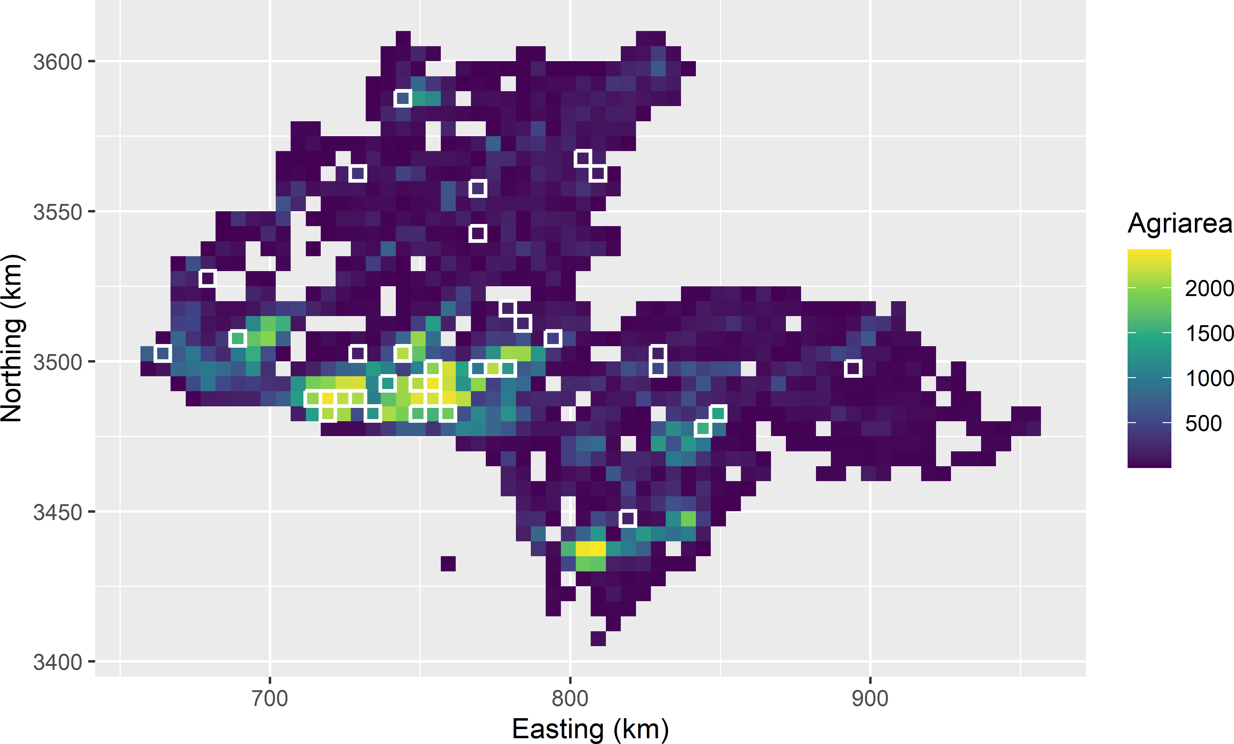
Figure 8.1: Sample of size 40 from Kandahar, selected with probabilities proportional to agricultural area with replacement. Four units are selected twice, so that the number of distinct units is 36.
The next code chunk shows how the population total of the poppy area can be estimated, using Equation (8.1), as well as the standard error of the estimator of the population total (square root of estimator of Equation (8.2)). As a first step, the observations are inflated, or expanded, through division of the observations by the selection probabilities of the corresponding units.
z_pexpanded <- mysample$poppy / mysample$p
tz <- mean(z_pexpanded)
se_tz <- sqrt(var(z_pexpanded) / n)
The estimated total equals 65,735 ha, with a standard error of 12,944 ha. The same estimates are obtained with package survey (Lumley 2021).
library(survey)
mysample$weight <- 1 / (mysample$p * n)
design_ppswr <- svydesign(id = ~ 1, data = mysample, weights = ~ weight)
svytotal(~ poppy, design_ppswr)
total SE
poppy 65735 12944In ppswr sampling, a sampling unit can be selected more than once, especially with large sampling fractions \(n/N\). This may decrease the sampling efficiency. With large sampling fractions, the alternative is pps sampling without replacement (ppswor), see next section.
The estimators of Equations (8.1) and (8.2) can also be used for infinite populations. For infinite populations, the probability that a unit is selected more than once is zero.
Exercises
- Write an R script to select a pps with replacement sample from Eastern Amazonia (
grdAmazoniain package sswr) to estimate the population mean of aboveground biomass (AGB), using log-transformed short-wave infrared radiation (SWIR2) as a size variable.- The correlation of AGB and lnSWIR2 is negative. The first step is to compute an appropriate size variable, so that the larger the size variable, the larger the selection probability. Multiply the lnSWIR2 values by -1. Then add a small value, so that the size variable becomes strictly positive.
- Select in a for-loop 1,000 times a ppswr sample of size 100 (\(n=100\)), and estimate from each sample the population mean of AGB with the pwr estimator (Hansen-Hurwitz estimator) and its sampling variance. Compute the variance of the 1,000 estimated population means and the mean of the 1,000 estimated variances. Make a histogram of the 1,000 estimated means.
- Compute the true sampling variance of the \(\pi\) estimator with simple random sampling with replacement and the same sample size.
- Compute the gain in precision by the ratio of the variance of the estimator of the mean with simple random sampling to the variance with ppswr.
8.2 Probability-proportional-to-size sampling without replacement
The alternative to pps sampling with replacement (ppswr) is pps sampling without replacement (ppswor). In ppswor sampling the inclusion probabilities are proportional to a size variable, not the draw-by-draw selection probabilities as in ppswr. For this reason, ppswor sampling is referred to as \(\pi\)ps sampling by Särndal, Swensson, and Wretman (1992). ppswor sampling starts with assigning target inclusion probabilities to all units in the population. With inclusion probabilities proportional to a size variable \(x\) the target inclusion probabilities are computed by \(\pi_k= n\;x_k/\sum_{j=1}^Nx_j,\; k = 1, \dots , N\).
8.2.1 Systematic pps sampling without replacement
Many algorithms are available for ppswor sampling, see Tillé (2006) for an overview. A simple, straightforward method is systematic ppswor sampling. Two subtypes can be distinguished, systematic ppswor sampling with fixed frame order and systematic ppswor sampling with random frame order (Rosén 1997). Given some order of the units, the cumulative sum of the inclusion probabilities is computed. Each population unit is then associated with an interval of cumulative inclusion probabilities. The larger the inclusion probability of a unit, the wider the interval. Then a random number from the uniform distribution is drawn, which serves as the start of a one-dimensional systematic sample of size \(n\) with an interval of 1. Finally, the units are determined for which the systematic random values are in the interval of cumulative inclusion probabilities, see Figure 8.2 for ten population units and a sample size of four. The units selected are 2, 5, 7, and 9. Note that the sum of the interval lengths equals the sample size. Further note that a unit cannot be selected more than once because the inclusion probabilities are \(<1\) and the sampling interval equals 1.
library(sampling)
set.seed(314)
N <- 10
n <- 4
x <- rnorm(N, mean = 20, sd = 5)
pi <- inclusionprobabilities(x, n)
print(data.frame(id = seq_len(N), x, pi))
id x pi
1 1 13.55882 0.3027383
2 2 23.63731 0.5277684
3 3 15.83538 0.3535687
4 4 16.48162 0.3679978
5 5 20.63624 0.4607613
6 6 18.32529 0.4091630
7 7 16.50655 0.3685545
8 8 20.06336 0.4479702
9 9 22.94495 0.5123095
10 10 11.15957 0.2491684cumsumpi <- c(0, cumsum(pi))
start <- runif(1, min = 0, max = 1)
sys <- 0:(n - 1) + start
print(units <- findInterval(sys, cumsumpi))[1] 2 5 7 9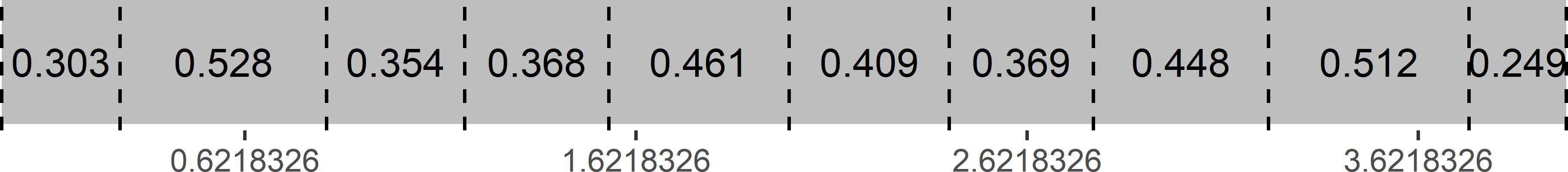
Figure 8.2: Systematic random sample along a line with unequal inclusion probabilities.
Sampling efficiency can be increased by ordering the units by the size variable (Figure 8.3). With this design, the third, fourth, fifth, and second units in the original frame are selected, with sizes 15.8, 16.5, 20.6, and 23.6, respectively. Ordering the units by size leads to a large within-sample and a small between-sample variance of the size variable \(x\). If the study variable is proportional to the size variable, this results in a smaller sampling variance of the estimator of the mean of the study variable. A drawback of systematic ppswor sampling with fixed order is that no unbiased estimator of the sampling variance exists.
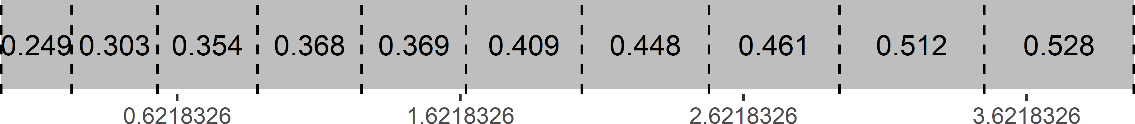
Figure 8.3: Systematic random sample along a line with unequal inclusion probabilities. Units are ordered by size.
A small simulation study is done next to see how much gain in precision can be achieved by ordering the units by size. A size variable \(x\) and a study variable \(z\) are simulated by drawing 1,000 values from a bivariate normal distribution with a correlation coefficient of 0.8. Function mvrnorm of package MASS (Venables and Ripley 2002) is used for the simulation.
library(MASS)
rho <- 0.8
mu1 <- 10; sd1 <- 2
mu2 <- 15; sd2 <- 4
mu <- c(mu1, mu2)
sigma <- matrix(
  data = c(sd1^2, rep(sd1 *  sd2 *  rho, 2), sd2^2),
  nrow = 2, ncol = 2)
N <- 1000
set.seed(314)
dat <- as.data.frame(mvrnorm(N, mu = mu, Sigma = sigma))
names(dat) <- c("z", "x")
head(dat)
z x
1 9.462930 9.149784
2 12.605847 17.306046
3 7.892686 11.979986
4 7.945021 12.567608
5 11.004325 15.165744
6 10.369943 13.258177Twenty units are selected by systematic ppswor sampling with random order and ordered by size. This is repeated 10,000 times.
The standard deviation of the 10,000 estimated means with systematic ppswor sampling with random order is 0.336, and when ordered by size 0.321. So, a small gain in precision is achieved through ordering the units by size. For comparison, I also computed the standard error for simple random sampling without replacement (SI) of the same size. The standard error with this basic sampling design is 0.424.
8.2.2 The pivotal method
Another interesting algorithm for ppswor sampling is the pivotal method (Deville and Tillé 1998). A nice adaptation of this algorithm, the local pivotal method, leading to samples with improved (geographical) spreading, is described in Section 9.2. In the pivotal method, the \(N\)-vector with inclusion probabilities is successively updated to a vector with indicators. If the indicator value for sampling unit \(k\) becomes 1, then this sampling unit is selected, if it becomes 0, then it is not selected. The updating algorithm can be described as follows:
- Select randomly two units \(k\) and \(l\) with \(0<\pi_k<1\) and \(0<\pi_l<1\).
- If \(\pi_k + \pi_l < 1\), then update the probabilities by
\[\begin{equation} (\pi^{\prime}_k,\pi^{\prime}_l)=\left\{ \begin{array}{cc} (0,\pi_k+\pi_l) & \;\;\;\text{with probability}\frac{\pi_l}{\pi_k+\pi_l} \\ (\pi_k+\pi_l,0) & \;\;\;\text{with probability}\frac{\pi_k}{\pi_k+\pi_l} \end{array} \right. \;, \tag{8.3} \end{equation}\]
and if \(\pi_k + \pi_l \geq 1\), update the probabilities by
\[\begin{equation} (\pi^{\prime}_k,\pi^{\prime}_l)=\left\{ \begin{array}{cc} (1,\pi_k+\pi_l-1) & \;\;\;\text{with probability}\frac{1-\pi_l}{2-(\pi_k+\pi_l)} \\ (\pi_k+\pi_l-1,1) & \;\;\;\text{with probability}\frac{1-\pi_k}{2-(\pi_k+\pi_l)} \end{array} \right.\;. \tag{8.4} \end{equation}\]
- Replace (\(\pi_k,\pi_l\)) by (\(\pi^{\prime}_k,\pi^{\prime}_l\)), and repeat the first two steps until each population unit is either selected (inclusion probability equals 1) or not selected (inclusion probability equals 0).
In words, when the sum of the inclusion probabilities is smaller than 1, the updated inclusion probability of one of the units will become 0, which means that this unit will not be sampled. The inclusion probability of the other unit will become the sum of the two inclusion probabilities, which means that the probability increases that this unit will be selected in one of the subsequent iterations. The probability of a unit of being excluded from the sample is proportional to the inclusion probability of the other unit, so that the larger the inclusion probability of the other unit, the larger the probability that it will not be selected.
When the sum of the inclusion probabilities of the two units is larger than or equal to 1, then one of the units is selected (updated inclusion probability is 1), while the inclusion probability of the other unit is lowered by 1 minus the inclusion probability of the selected unit. The probability of being selected is proportional to the complement of the inclusion probability of the other unit. After the inclusion probability of a unit has been updated to either 0 or 1, this unit cannot be selected anymore in the next iteration.
With this ppswor design, the population total can be estimated by the \(\pi\) estimator, Equation (2.2). The \(\pi\) estimator of the mean is simply obtained by dividing the estimator for the total by the population size \(N\).
An alternative estimator of the population mean is the ratio estimator, also known as the Hájek estimator:
\[\begin{equation} \hat{\bar{z}}_{\text{Hajek}}=\frac{\sum_{k \in \mathcal{S}} w_k z_k}{\sum_{k \in \mathcal{S}} w_k} \;, \tag{8.5} \end{equation}\]
with \(w_k = 1/\pi_k\). The denominator is an estimator of the population size \(N\). The Hájek estimator of the population total is obtained by multiplying the Hájek estimator of the mean with the population size \(N\). Recall that the ratio estimator of the population mean was presented before in the chapters on systematic random sampling (Equation (5.4)), cluster random sampling with simple random sampling of clusters (Equation (6.12)), and two-stage cluster random sampling with simple random sampling of PSUs. These sampling designs have in common that the sample size (for cluster random sampling, the number of SSUs) is random.
Various functions in package sampling (Tillé and Matei 2021) can be used to select a ppswor sample. In the code chunk below, I use function UPrandompivotal. With this function, the order of the population units is randomised before function UPpivotal is used. Argument pi is a numeric with the inclusion probabilities. These are computed with function inclusionprobabilities. Recall that \(\pi_k= n\;x_k/t(x)\). The sum of the inclusion probabilities should be equal to the sample size \(n\). Function UPpivotal returns a numeric of length \(N\) with elements 1 and 0, 1 if the unit is selected, 0 if it is not selected.
library(sampling)
n <- 40
pi <- inclusionprobabilities(grdKandahar$agri, n)
set.seed(314)
sampleind <- UPrandompivotal(pik = pi)
mysample <- data.frame(grdKandahar[sampleind == 1, ], pi = pi[sampleind == 1])
nrow(mysample)
[1] 39As can be seen, not 40 but only 39 units are selected. The reason is that function UPrandompivotal uses a very small number that can be set with argument eps. If the updated inclusion probability of a unit is larger than the complement of this small number eps, the unit is treated as being selected. The default value of eps is \(10^{-6}\). If we replace sampleind == 1 by sampleind > 1 - eps, 40 units are selected.
eps <- 1e-6
mysample <- data.frame(
  grdKandahar[sampleind > 1 - eps, ], pi = pi[sampleind > 1 - eps])
nrow(mysample)
[1] 40The total poppy area can be estimated from the ppswor sample by
tz_HT <- sum(mysample$poppy / mysample$pi)
N <- nrow(grdKandahar)
tz_Hajek <- N * sum(mysample$poppy / mysample$pi) / sum(1 / mysample$pi)
The total poppy area as estimated with the \(\pi\) estimator equals 88,501 ha. The Hájek estimator results in a much smaller estimated total: 59,993 ha.
The \(\pi\) estimate can also be computed with function svytotal of package survey, which also provides an approximate estimate of the standard error. Various methods are implemented in function svydesign for approximating the standard error. These methods differ in the way the pairwise inclusion probabilities are approximated from the unitwise inclusion probabilities. These approximated pairwise inclusion probabilities are then used in the \(\pi\) variance estimator or the Yates-Grundy variance estimator. In the next code chunks, Brewer’s method is used, see option 2 of Brewer’s method in Berger (2004), as well as Hartley-Rao’s method for approximating the variance.
library(survey)
design_ppsworbrewer <- svydesign(
  id = ~ 1, data = mysample, pps = "brewer", fpc = ~ pi)
svytotal(~ poppy, design_ppsworbrewer)
total SE
poppy 88501 14046p2sum <- sum(mysample$pi^2) / n
design_ppsworhr <- svydesign(
id = ~ 1, data = mysample, pps = HR(p2sum), fpc = ~ pi)
svytotal(~ poppy, design_ppsworhr) total SE
poppy 88501 14900In package samplingVarEst (Escobar, Zamudio, and Munoz Rosas 2019), also various functions are available for approximating the variance: VE.Hajek.Total.NHT, VE.HT.Total.NHT, and VE.SYG.Total.NHT. The first variance approximation is the Hájek-Rosén variance estimator, see equation (4.3) in Rosén (1997). The latter two functions require the pairwise inclusion probabilities, which can be estimated by function Pkl.Hajek.s.
library(samplingVarEst)
se_tz_Hajek <- sqrt(VE.Hajek.Total.NHT(mysample$poppy, mysample$pi))
pikl <- Pkl.Hajek.s(mysample$pi)
se_tz_HT <- sqrt(VE.HT.Total.NHT(mysample$poppy, mysample$pi, pikl))
se_tz_SYG <- sqrt(VE.SYG.Total.NHT(mysample$poppy, mysample$pi, pikl))
The three approximated standard errors are 14,045, 14,068, and 14,017 ha. The differences are small when related to the estimated total.
Figure 8.4 shows the approximated sampling distribution of estimators of the total poppy area with ppswor sampling and simple random sampling without replacement of size 40, obtained by repeating the random sampling with each design and estimation 10,000 times. With the ppswor samples, the total poppy area is estimated by the \(\pi\) estimator and the Hájek estimator. For each ppswor sample, the variance of the \(\pi\) estimator is approximated by the Hájek-Rosén variance estimator (using function VE.Hajek.Total.NHT of package samplingVarEst).
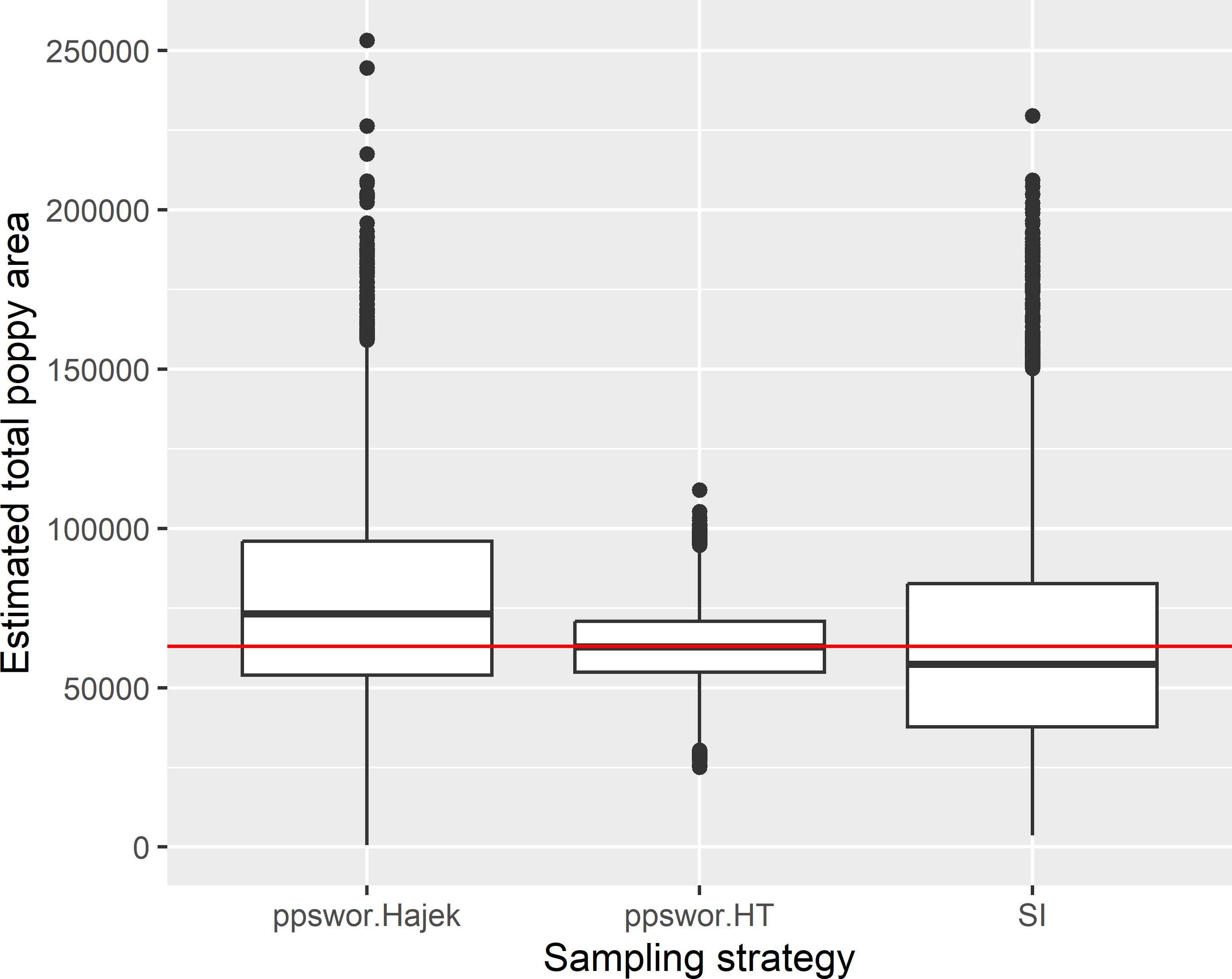
Figure 8.4: Approximated sampling distribution of the \(\pi\) estimator (ppswor.HT) and the Hájek estimator (ppswor.Hajek) of the total poppy area (ha) in Kandahar with ppswor sampling of size 40, and of the \(\pi\) estimator with simple random sampling without replacement (SI) of size 40.
Sampling design ppswor in combination with the \(\pi\) estimator is clearly much more precise than simple random sampling. The standard deviation of the 10,000 \(\pi\) estimates of the total poppy area with ppswor equals 11,684 ha. The average of the square root of the Hájek-Rosén approximated variances equals 12,332 ha.
Interestingly, with ppswor sampling the variance of the 10,000 Hájek estimates is much larger than that of the \(\pi\) estimates. The standard deviation of the 10,000 Hájek estimates with ppswor sampling is about equal to that of the \(\pi\) estimates with simple random sampling: 31,234 ha and 33,178 ha, respectively.
Exercises
- A field with poppy was found outside Kandahar in a selected sampling unit crossing the boundary. Should this field be included in the sum of the poppy area of that sampling unit?
- In another sampling unit, a poppy field was encountered in Kandahar but in the area represented as non-agricultural in the GIS map. Should this field be included in the sum of that sampling unit?