Chapter 23 Model-based optimisation of the sampling pattern

In Chapter 22 a model of the spatial variation is used to optimise the spacing of a regular grid. The grid spacing determines the number of grid points within the study area, so optimisation of the grid spacing is equivalent to optimisation of the sample size of a square grid.

This chapter is about optimisation of the spatial coordinates of the sampling units given the sample size. So, we are searching for the optimal spatial sampling pattern of a fixed number of sampling units. The constraint of sampling on a regular grid is dropped. In general, the optimal spatial sampling pattern is irregular. Similar to spatial coverage sampling (Section 17.2), we search for the optimal sampling pattern through minimisation of an explicit criterion. In spatial coverage sampling, the minimisation criterion is the mean squared shortest distance (MSSD) which is minimised by k-means. In this chapter the minimisation criterion is the mean kriging variance (MKV) or a quantile of the kriging variance. Algorithm k-means cannot be used for minimising this criterion, as it uses (standardised) distances between cluster centres (the sampling locations) and the nodes of a discretisation grid, and the kriging variance is not a simple linear function of these distances. A different optimisation algorithm is needed. Here, spatial simulated annealing is used which is explained in the next subsection. Non-spatial simulated annealing was used before in conditioned Latin hypercube sampling using package clhs (Chapter 19).

23.1 Spatial simulated annealing

Inspired by the potentials of optimisation through simulated annealing (Kirkpatrick, Gelatt, and Vecchi 1983), van Groenigen and Stein (1998) proposed to optimise the sampling pattern by spatial simulated annealing (SSA), see also van Groenigen, Siderius, and Stein (1999) and van Groenigen, Pieters, and Stein (2000). This is an iterative, random search procedure, in which a sequence of samples is generated. A newly proposed sample is obtained by slightly modifying the current sample. One sampling location of the current sample is randomly selected, and this location is shifted to a random location within the neighbourhood of the selected location.

The minimisation criterion is computed for the proposed sample and compared with that of the current sample. If the criterion of the proposed sample is smaller, the sample is accepted. If the criterion is larger, the sample is accepted with a probability equal to

\[\begin{equation} P = e^{\frac{-\Delta}{T}}\;, \tag{23.1} \end{equation}\]

with \(\Delta\) the increase of the criterion and \(T\) the “temperature”.

The name of this parameter shows the link with annealing in metallurgy. Annealing is a heat treatment of a material above its recrystallisation temperature. Simulated annealing mimics the gradual cooling of metal alloys, resulting in an optimum or near-optimum structure of the atoms in the alloy.

The larger the value of \(T\), the larger the probability that a proposed sample with a given increase of the criterion is accepted (Figure 23.1). The temperature \(T\) is stepwise decreased during the optimisation: \(T_{k+1} = \alpha T_k\). In Figure 23.1 \(\alpha\) equals 0.9. The effect of decreasing the temperature is that the acceptance probability of worse samples decreases during the optimisation and approaches 0 towards the end of the optimisation. Note that the temperature remains constant during a number of iterations, referred to as the chain length. In Figure 23.1 this chain length equals 100 iterations. Finally, a stopping criterion is required. Various stopping criteria are possible; one option is to set the maximum numbers of chains with no improvement. \(T, \alpha\), the chain length, and the stopping criterion are annealing schedule parameters that must be chosen by the user.

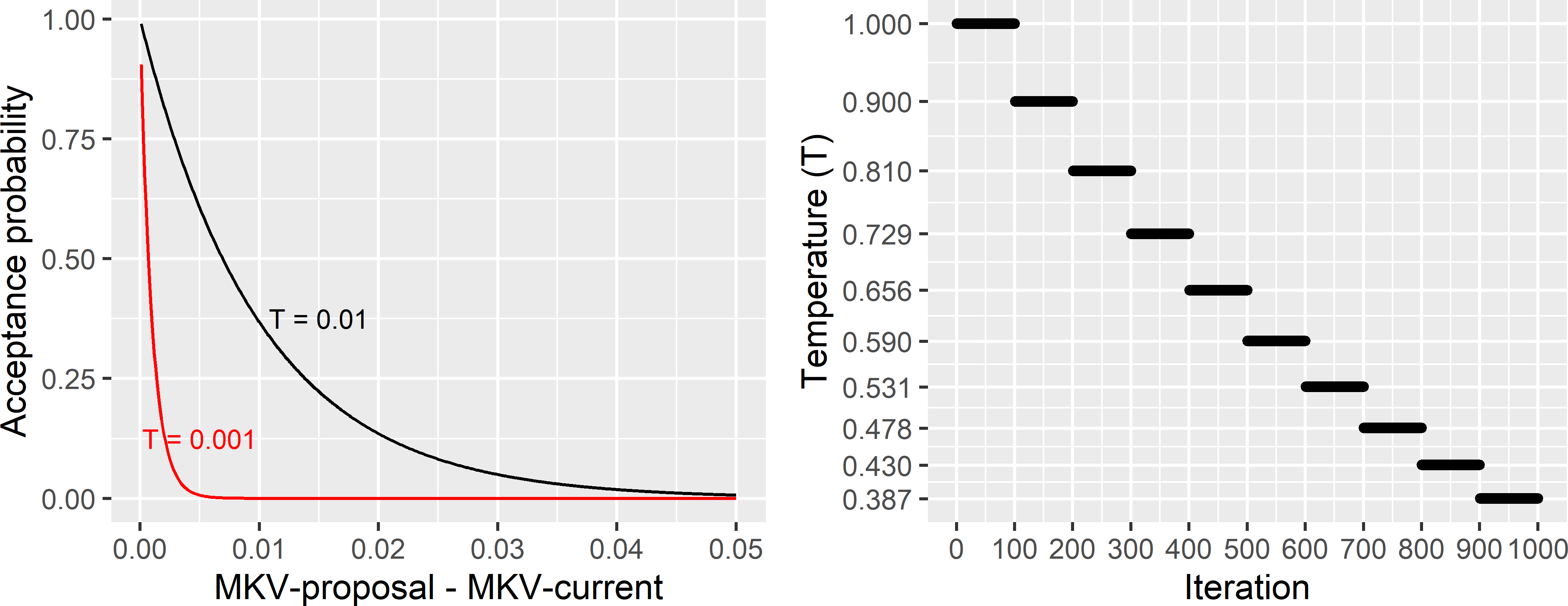
Figure 23.1: Acceptance probability as a function of the change in the mean kriging variance (MKV) used as a minimisation criterion, and cooling schedule in spatial simulated annealing. For negative changes (MKV of proposed sample smaller than of current sample) the acceptance probability equals 1.

23.2 Optimising the sampling pattern for ordinary kriging

In ordinary kriging (OK), we assume a constant model-mean. No covariates are available that are related to the study variable. Optimisation of the sampling pattern for OK is illustrated with the Cotton Research Farm in Uzbekistan which was used before to illustrate spatial response surface sampling (Chapter 20). The spatial coordinates of 50 sampling locations are optimised for mapping of the soil salinity (as measured by the electrical conductivity, ECe, of the soil) by OK. In this section, the coordinates of the sampling points are optimised for OK. In Section 23.3 this is done for kriging with an external drift. In that section, a map of interpolated electromagnetic (EM) induction measurements is used to further optimise the coordinates of the sampling points.

Model-based optimisation of the sampling pattern for OK requires as input a semivariogram of the study variable. For the Cotton Research Farm, I used the ECe (dS m^-1) data collected in eight surveys in the period from 2008 to 2011 at 142 points to estimate this semivariogram (Akramkhanov, Brus, and Walvoort 2014). The ECe data are natural-log transformed. The sample semivariogram is shown in Figure 23.2. The R code below shows how I fitted the semivariogram model with function nls (“non-linear least squares”) of the stat package. I did not use function fit.variogram of the gstat package (E. J. Pebesma 2004), because this function requires the output of function variogram as input, whereas the sample semivariogram is here computed in a different way.

The sample semivariogram is computed by first estimating sample semivariograms for each of the eight surveys separately, followed by computing weighted averages of semivariances and distances per lag, using the numbers of pairs as weights (R code not shown).

The semivariogram parameters as estimated by nls are then used to define a semivariogram model of class variogramModel of package gstat, using function vgm. This is done because function optimMKV requires a semivariogram model of this class, see hereafter. As already mentioned in Chapter 22, in practice we often do not have legacy data from which we can estimate the semivariogram, and a best guess of the semivariogram then must be made.

library(gstat)
res_nls <- nls(semivar ~ nugget + psill * (1 - exp(-h / range)),
  start = list(nugget = 0.1, psill = 0.4, range = 200), weights = somnp)
vgm_lnECe <- vgm(model = "Exp", nugget = coef(res_nls)[1],
  psill = coef(res_nls)[2], range = coef(res_nls)[3])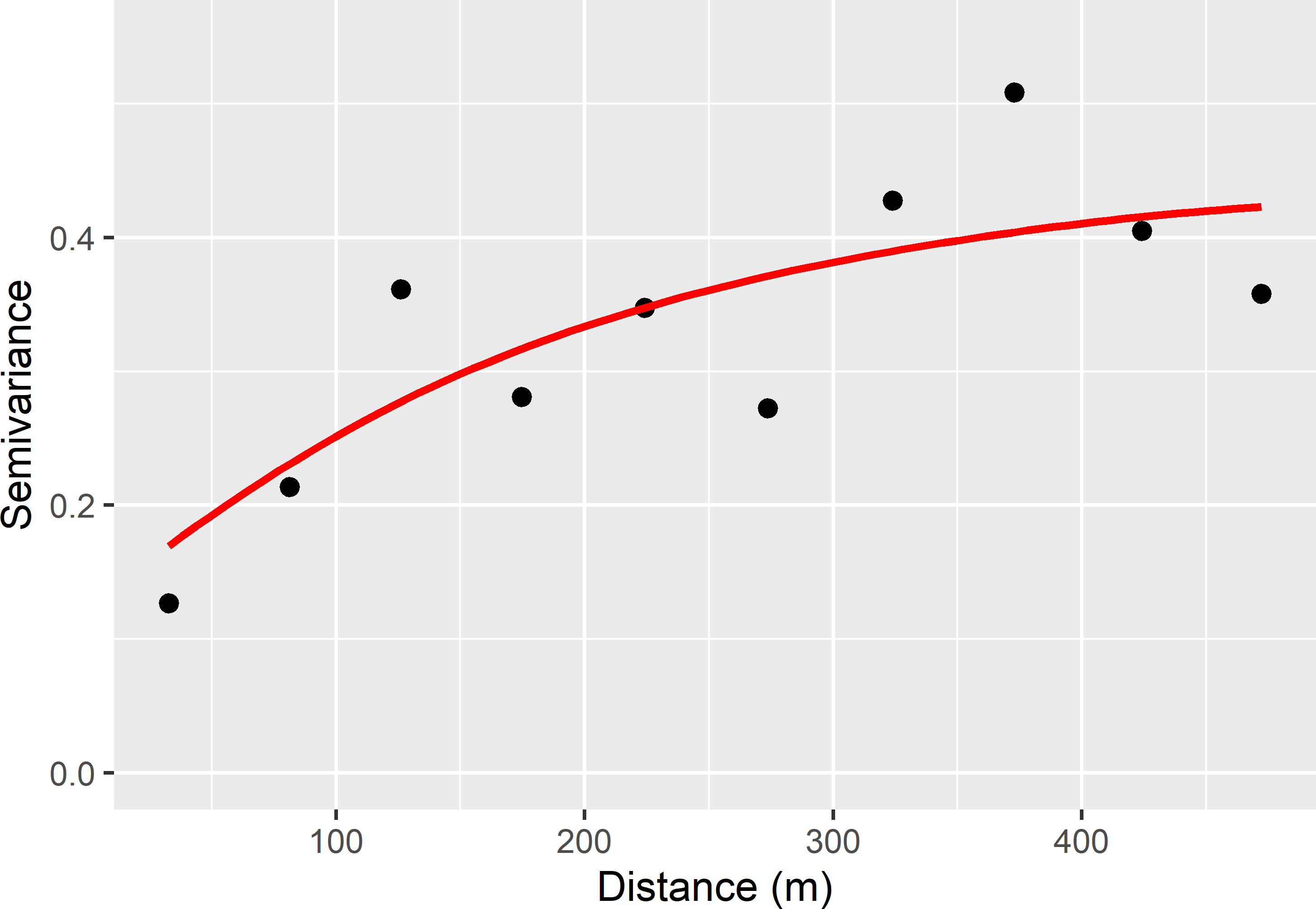

Figure 23.2: Sample semivariogram and fitted exponential model of lnECe at the Cotton Research Farm.

The estimated semivariogram parameters are shown in Table 23.1. The nugget-to-sill ratio is about 1/4, and the effective range is about 575 m (three times the distance parameter of an exponential model).

The coordinates of the sampling points are optimised with function optimMKV of package spsann (Samuel-Rosa 2019)¹⁴. First, the candidate sampling points are specified by the nodes of a grid discretising the population. As explained hereafter, this does not necessarily imply that the population is treated as a finite population. Next, the parameters of the annealing schedule are set. Note that both the initial acceptance rate and the initial temperature are set, which may seem weird as the acceptance rate is a function of the temperature, see Equation (23.1). The optimisation stops when an initial temperature is chosen leading to an acceptance rate outside the interval specified with argument initial.acceptance. If the acceptance rate is smaller than the lower bound of the interval, a larger value for the initial temperature must be chosen; if the rate is larger than the upper bound, a smaller initial temperature must be chosen. Arguments chain.length and stopping of function scheduleSPSANN are multipliers. So, for a chain length of five, the number of iterations equals \(5n\), with \(n\) the sample size.

During the optimisation, a sample is perturbed by replacing one randomly selected point of the current sample by a new point. This selection of the new point is done in two steps. In the first step, one node of the discretisation grid (specified with argument candi) is randomly selected. Only the nodes within a neighbourhood defined by x.min, x.max, y.min, and y.max can be selected. The nodes within this neighbourhood have equal probability of being selected. In the second step, one point is selected within a grid cell with the selected node at its centre and a side length specified with argument cellsize. So, it is natural to set cellsize to the spacing of the discretisation grid. With cellsize = 0, the sampling points are restricted to the nodes of the discretisation grid.

library(spsann)
candi <- grdCRF[, c("x", "y")]
schedule <- scheduleSPSANN(
  initial.acceptance = c(0.8,0.95),
  initial.temperature = 0.004, temperature.decrease = 0.95,
  chains = 500, chain.length = 2, stopping = 10, cellsize = 25)

The R code for optimising the sampling pattern is as follows.

set.seed(314)
res <- optimMKV(
  points = 50, candi = candi,
  vgm = vgm_lnECe, eqn = z ~ 1,
  schedule = schedule, nmax = 20, 
  plotit = FALSE, track = TRUE)
mysample <- res$points
trace <- res$objective$energy

The spatial pattern of the sample in Figure 23.3 and the trace of the MKV in Figure 23.4 suggest that we are close to the global optimum.

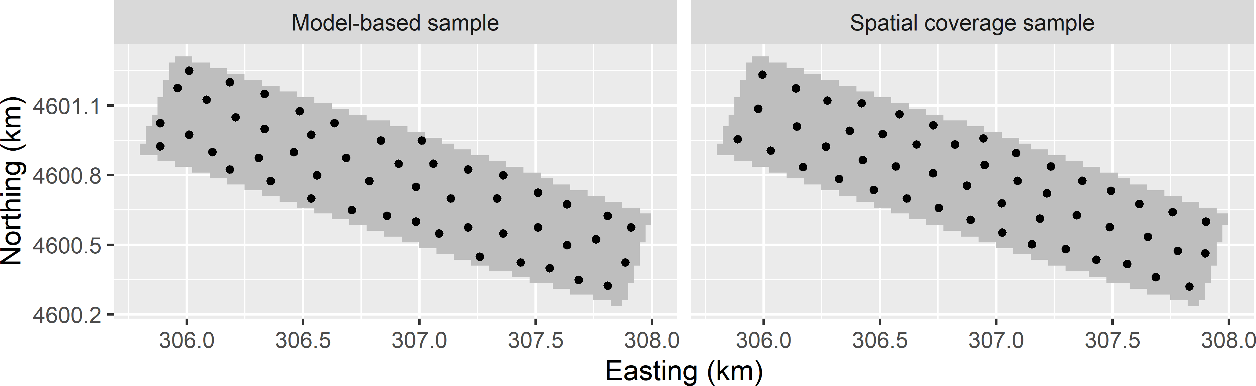
Figure 23.3: Optimised sampling pattern for the mean variance of OK predictions of lnECe (model-based sample) and spatial coverage sample of the Cotton Research Farm.

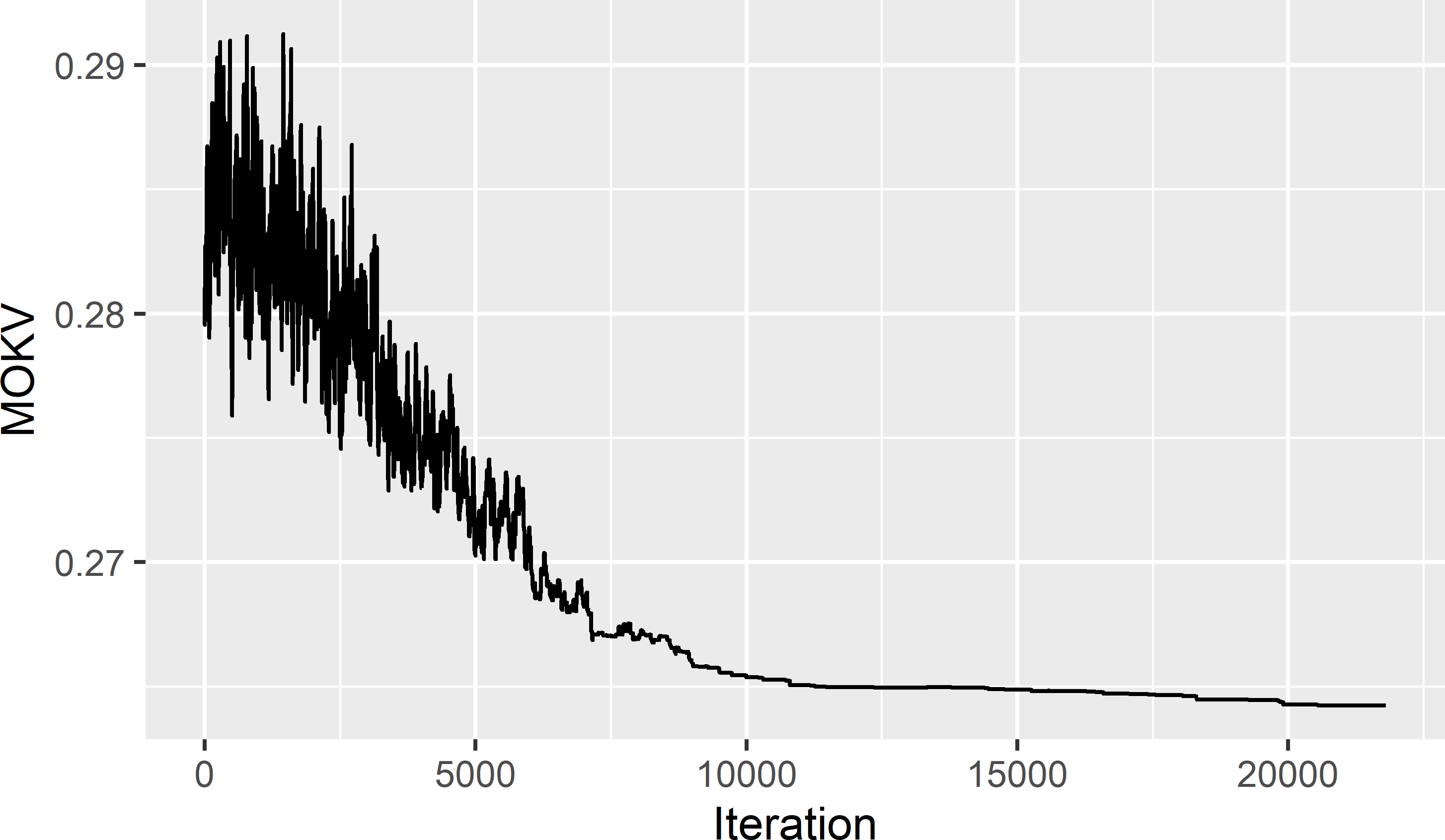
Figure 23.4: Trace of the mean ordinary kriging variance (MOKV).

For comparison I also computed a spatial coverage sample of the same size. The spatial patterns of the two samples are quite similar (Figure 23.3). The MKV of the spatial coverage sample equals 0.2633 (dS m^-1)², whereas for the model-based sample the MKV equals 0.2642 (dS m^-1)². So, no gain in precision is achieved by the model-based optimisation of the sampling pattern compared to spatial coverage sampling. With cellsize = 0 the minimised MKV is slightly smaller: 0.2578 (dS m^-1)². This outcome is in agreement with the results reported by Brus, de Gruijter, and van Groenigen (2007).

Instead of the mean OK variance (MOKV), we may prefer to use some quantile of the cumulative distribution function of the OK variance as a minimisation criterion. For instance, if we use the 0.90 quantile as a criterion, we are searching for the sampling locations so that the 90th percentile (P90) of the OK variance is minimal. This can be done with function optimUSER of package spsann. The objective function to be minimised can be passed to this function with argument fun. In this case the objective function is as follows.

QOKV <- function(points, esample, model, nmax, prob) {
  points <- as.data.frame(points)
  coordinates(points) <- ~ x + y
  points$dum <- 1
  res <- krige(
    formula = dum ~ 1,
    locations = points,
    newdata = esample,
    model = model,
    nmax = nmax,
    debug.level = 0)
  quantile(res$var1.var, probs = prob)
}

The next code chunk shows how this objective function can be minimised.

mysample_eval <- candi
coordinates(mysample_eval) <- ~ x + y
set.seed(314)
res <- optimUSER(
  points = 50, candi = candi,
  fun = QOKV,
  esample = mysample_eval,
  model = vgm_lnECe,
  nmax = 20, prob = 0.9,
  schedule = schedule)

Argument esample specifies a SpatialPoints object with the evaluation points, i.e., the points at which the kriging variance is computed. Above I used all candidate sampling points as evaluation points. Computing time can be reduced by selecting a coarser square grid with evaluation points. The number of points used in kriging is specified with argument nmax, and the probability of the cumulative distribution function of the kriging variance is specified with argument prob. Optimisation of the sampling pattern for a quantile of the OK variance is left as an exercise.

Exercises

1. Write an R script to optimise the spatial coordinates of 16 points in a square for OK. First, create a discretisation grid of 20 \(\times\) 20 nodes. Use an exponential semivariogram without nugget, with a sill of 2, and a distance parameter of four times the spacing of the discretisation grid. Optimise the sampling pattern with SSA (using functions scheduleSPSANN and optimMKV of package spsann).
   • Check whether the optimisation has converged by plotting the trace of the optimisation criterion MKV.
   • Based on the coordinates of the sampling points, do you think the sample is the global optimum, i.e., the sample with the smallest possible MKV?
     
2. Write an R script to optimise the sampling pattern of 50 points, using the P90 of the variance of OK predictions of lnECe on the Cotton Research Farm as a minimisation criterion. Use the semivariogram parameters of Table 23.1. Compare the optimised sample with the sample optimised with the mean OK variance (shown in Figure 23.3).

23.3 Optimising the sampling pattern for kriging with an external drift

If we have one or more covariates that are linearly related to the study variable, the study variable can be mapped by kriging with an external drift (KED). A requirement is that we have maps of the covariates so that, once we have estimated the parameters of the model for KED from the data collected at the optimised sample, these covariate maps can be used to map the study variable (see Equation (21.21)).

Optimisation of the sampling pattern for KED requires as input the semivariogram of the residuals. Besides, we must decide on the covariates for the model-mean. Note that we do not need estimates of the regression coefficients associated with the covariates as input, but just which combination of covariates we want to use for modelling the model-mean of the study variable.

Optimisation of the sampling pattern for KED is illustrated with the Cotton Research Farm. The interpolated natural log of the EM data (with transmitter at 1 m) is used as a covariate, see Figure 20.1. The data for fitting the model are in data file sampleCRF. The parameters of the residual semivariogram are estimated by restricted maximum likelihood (REML), see Subsection 21.5.2.

At several points, multiple pairs of observations of the study variable ECe and the covariate EM have been made. These calibration data have exactly the same spatial coordinates. This leads to problems with REML estimation. The covariance matrix is not positive definite, so that it cannot be inverted. To solve this problem, I jittered the coordinates of the sampling points by a small amount.

library(geoR)
sampleCRF$lnEM100 <- log(sampleCRF$EMv1m)
sampleCRF$x <- jitter(sampleCRF$x, amount = 0.001)
sampleCRF$y <- jitter(sampleCRF$y, amount = 0.001)
dGeoR <- as.geodata(obj = sampleCRF, header = TRUE,
  coords.col = c("x", "y"), data.col = "lnECe", covar.col = "lnEM100")
vgm_REML <- likfit(geodata = dGeoR, trend = ~ lnEM100,
  cov.model = "exponential", ini.cov.pars = c(0.1, 200),
  nugget = 0.1, lik.method = "REML", messages = FALSE)

The REML estimates of the parameters of the residual semivariogram are shown in Table 23.1. The estimated sill (sum of nugget and partial sill) of the residual semivariogram is substantially smaller than that of lnECe, showing that the linear model for the model-mean explains a considerable part of the spatial variation of lnECe.

Table 23.1: Estimated parameters of an exponential semivariogram for lnECe (estimated by method-of-moments) and for the residuals of a linear regression model for lnECe using lnEM100cm as a predictor (estimated by REML).

Variable	Nugget	Partial sill	Distance parameter (m)
lnECe	0.116	0.336	192
residuals	0.126	0.083	230

To optimise the sampling pattern for KED, using the mean KED variance as a minimisation criterion, a data frame with the covariates at the candidate sampling points must be specified with argument covars. The formula for the model-mean is specified with argument eqn.

set.seed(314)
res <- optimMKV(
  points = 50, candi = candi, covars = grdCRF,
  vgm = vgm_REML_gstat, eqn = z ~ lnEM100cm,
  schedule = schedule, nmax = 20,
  plotit = FALSE, track = FALSE)

Figure 23.5 shows the optimised locations of a sample of 50 points. This clearly shows the irregular spatial pattern of the sampling points induced by the covariate lnEM100cm. Computing time was substantial: 35.06 minutes (processor AMD Ryzen 5, 16 GB RAM).

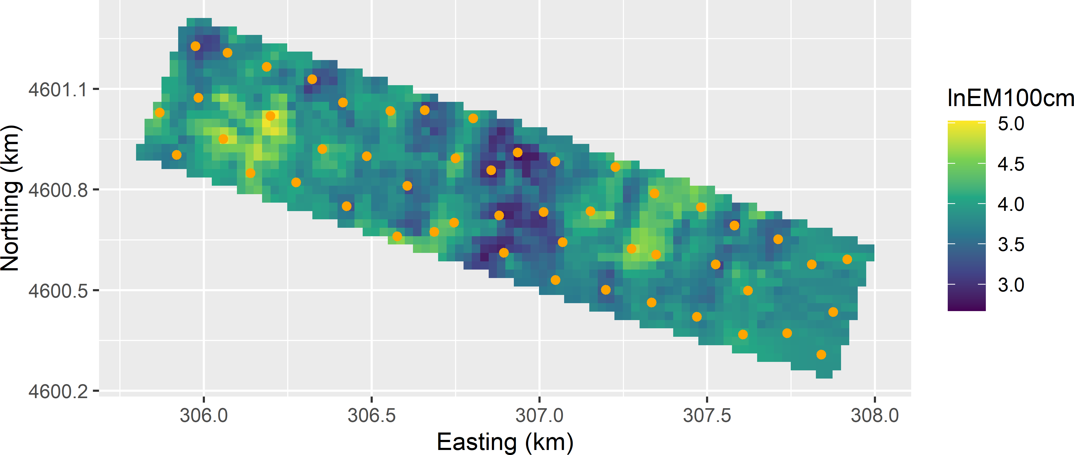
Figure 23.5: Optimised sampling pattern for KED of lnECe at the Cotton Research Farm, using lnEM100cm as a covariate.

Comparing the population and sample histograms of the covariate clearly shows that locations with small and large values for the covariate are preferentially selected (Figure 23.6). The optimised sampling pattern is a compromise between spreading in geographic space and covariate space, see also Heuvelink, Brus, and Gruijter (2007) and Brus and Heuvelink (2007). More precisely, locations are selected by spreading them throughout the study area, while accounting for the values of the covariates at the selected locations, in a way that locations with covariate values near the minimum and maximum are preferred. This can be explained by noting that the variance of the KED prediction error can be decomposed into two components: the variance of the interpolated residuals and the variance of the estimator of the model-mean, see Section 21.3. The contribution of the first variance component is minimised through geographical spreading, that of the second component by selecting locations with covariate values near the minimum and maximum.

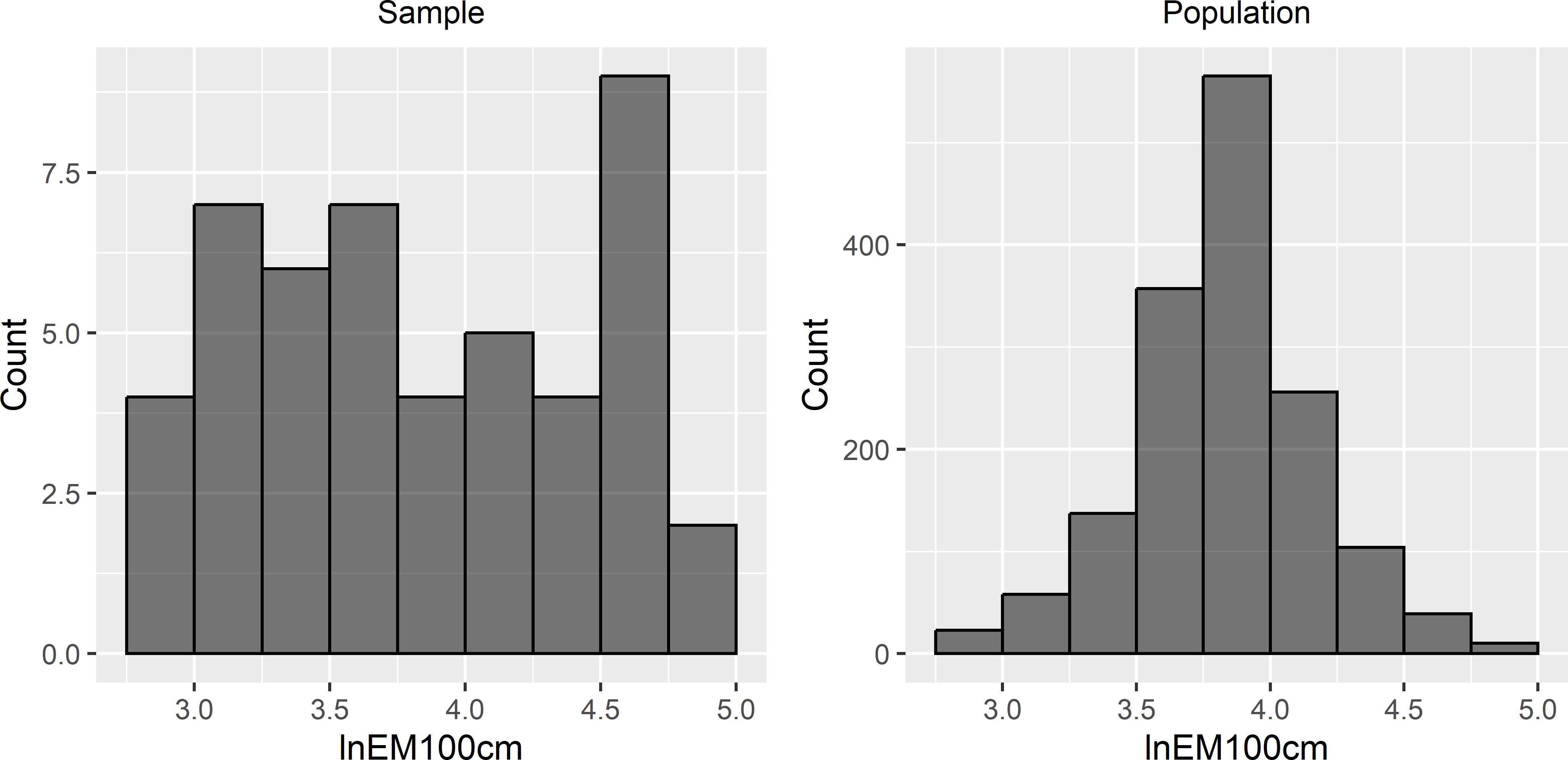
Figure 23.6: Sample frequency distribution and population frequency distribution of lnEM100cm used as covariate in model-based optimisation of the sampling pattern for mapping with KED.

A sample with covariate values close to the minimum and maximum only is not desirable if we do not want to rely on the assumption of a linear relation between the study variable and the covariates. To identify a non-linear relation, locations with intermediate covariate values are needed. Optimisation using a semivariogram with clear spatial structure leads to geographical spreading of the sampling units, so that most likely also locations with intermediate covariate values are selected.

When one or more covariates are used in optimisation of the sampling pattern but not used in KED once the data are collected, the sample is suboptimal for the model used in prediction. Inversely, ignoring a covariate in optimisation of the sampling pattern while using this covariate as a predictor also leads to suboptimal samples. The selection of covariates to be used in sampling design therefore should be done with care. Besides, as we will see in the next exercise, the nugget of the residual semivariogram has a strong effect on the optimised sampling pattern, stressing the importance of a reliable prior estimate of this semivariogram parameter.

Exercises

3. Write an R script to optimise the sampling pattern of 16 points in a square for KED. Use the \(x\)-coordinate as a covariate. First, create a discretisation grid of 20 \(\times\) 20 nodes. Use an exponential residual semivariogram without nugget, with a sill of 2, and a distance parameter of four times the spacing of the discretisation grid. Optimise the sampling pattern with SSA (using functions scheduleSPSANN and optimMKV of package spsann).
   • What do you think of the spatial coverage of the optimised sample? Compare the sample with the optimised sample for OK, see exercise of Section 23.2.
   • Repeat the optimisation using a residual semivariogram with a nugget of 1.5 and a partial sill of 0.5. Note that the sill is again 2, as before.
   • Compare the optimised sample with the previous sample. What is the most striking difference?
   • How will the optimised sample look with a pure nugget semivariogram? Check your assumption using such semivariogram in SSA.

23.4 Model-based infill sampling for ordinary kriging

Similar to spatial infill sampling using MSSD as a minimisation criterion (Section 17.3), we may design a model-based infill sample. Package spsann can be used for this, using argument points of function optimMKV.

In Section 22.1 the legacy data of West-Amhara were used to estimate the parameters of a spherical semivariogram for the SOM concentration. The estimated parameters are shown in Table 22.1. The maximum likelihood estimates are used in this section to optimise the spatial coordinates of the infill sample.

In the next code chunk, a list is created containing a data frame with the coordinates of the fixed points (specified with subargument fixed) and an integer of the number of additional points to be selected (specified with subargument free). The list is passed to function optimMKV with argument points. For kriging, I reduced the number of legacy points by keeping one point only per grid cell of 1 km \(\times\) 1 km. This is done with function remove.duplicates of package sp.

library(sp)
coordinates(sampleAmhara) <- ~ s1 + s2
legacy <- remove.duplicates(sampleAmhara, zero = 1, remove.second = TRUE)
pnts <- list(fixed = coordinates(legacy), free = 100)
candi <- grdAmhara[, c("s1", "s2")]
names(candi) <- c("x", "y")

The number of points used in kriging can be passed to function optimMKV with argument nmax.

set.seed(314)
vgm_ML_gstat <- vgm(model = "Sph", psill = vgm_ML$sigmasq,
  range = vgm_ML$phi, nugget = vgm_ML$nugget)
res <- optimMKV(
  points = pnts, candi = candi,
  vgm = vgm_ML_gstat, eqn = z ~ 1,
  nmax = 20, schedule = schedule, track = FALSE)
infillSample <- res$points %>%
  filter(free == 1)

Figure 23.7 shows a model-based infill sample of 100 points for OK of the soil organic matter (SOM) concentration (dag kg^-1) throughout West-Amhara. Comparison of the model-based infill sample with the spatial infill sample of Figure 17.5 shows that in a wider zone on both sides of the roads no new sampling points are selected. This can be explained by the large range, 36.9 km, of the semivariogram.

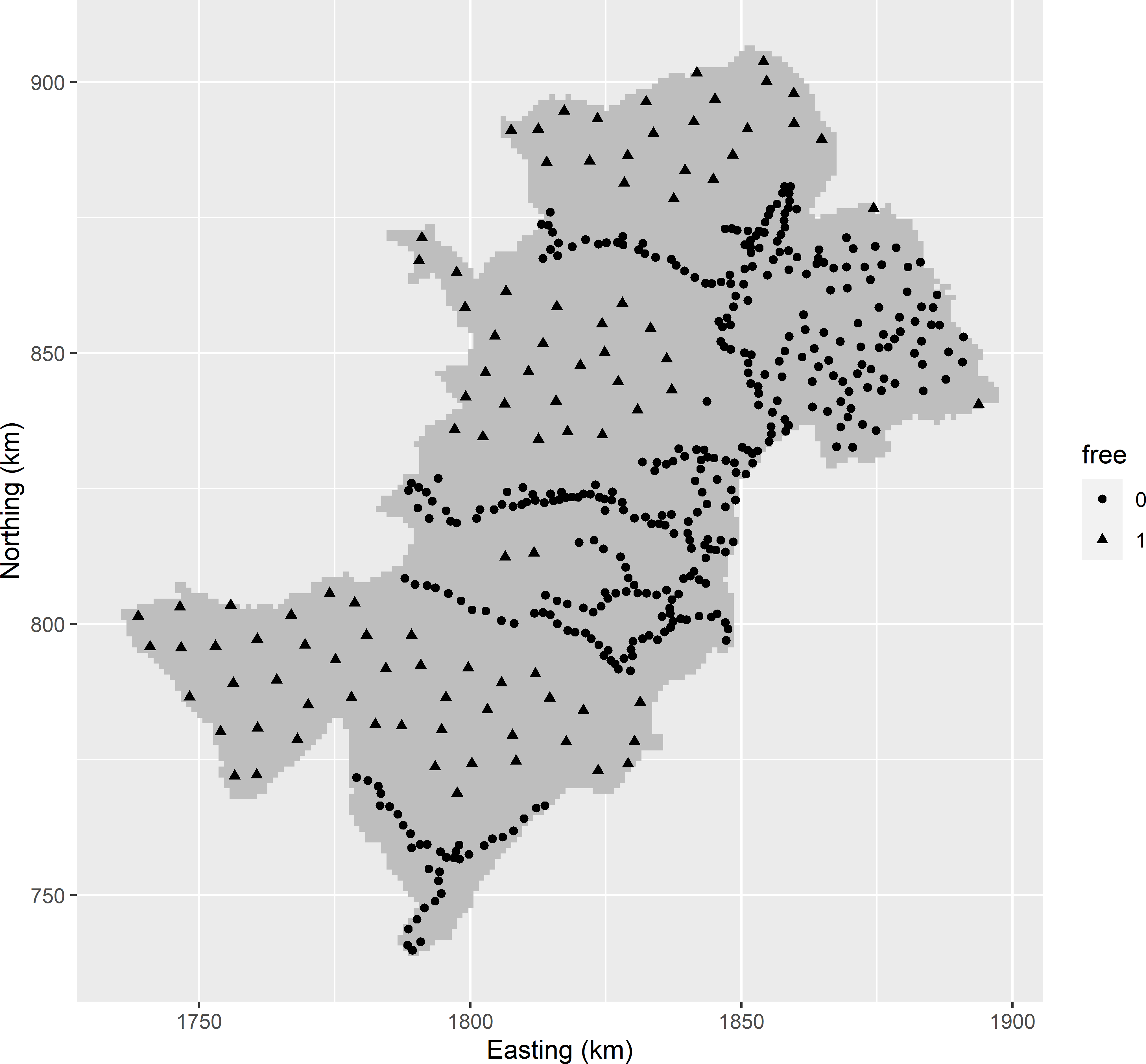
Figure 23.7: Model-based infill sample for OK of the SOM concentration throughout West-Amhara. Legacy units have free-value 0; infill units have free-value 1.

23.5 Model-based infill sampling for kriging with an external drift

For West-Amhara, maps of covariates are available that can be used in KED, see Section 22.4. The prediction error variance with KED is partly determined by the covariate values (see Section 23.3), and therefore, when filling in the undersampled areas, locations with extreme values for the covariates are preferably selected. In Section 22.4 the legacy data were used to estimate the residual semivariogram by REML, see Table 22.2. In the next code chunk, the estimated parameters of the residual semivariogram are used to optimise the spatial pattern of an infill sample of 100 points for mapping the SOM concentration throughout West-Amhara by KED, using elevation (dem), NIR-reflectance (rfl_NIR), red-reflectance (rfl_red), and land surface temperature (lst) as predictors for the model-mean.

covars <- grdAmhara[, c("dem", "rfl_NIR", "rfl_red", "lst")]
vgm_REML_gstat <- vgm(model = "Sph", psill = vgm_REML$sigmasq,
  range = vgm_REML$phi, nugget = vgm_REML$nugget)
set.seed(314)
res <- optimMKV(
  points = pnts, candi = candi, covars = covars,
  vgm = vgm_REML_gstat,
  eqn = z ~ dem + rfl_NIR + rfl_red + lst,
  nmax = 20, schedule = schedule, track = TRUE)

Figure 23.8 shows the optimised sample. Again the legacy points are avoided, but the infill sampling of the undersampled areas is less uniform compared to Figure 23.7. Spreading in geographical space is less important than with OK because the residual semivariogram has a much smaller range (Table 22.2). Spreading in covariate space does not play any role with OK, whereas with KED selecting locations with extreme values for the covariates is important to minimise the uncertainty about the estimated model-mean.

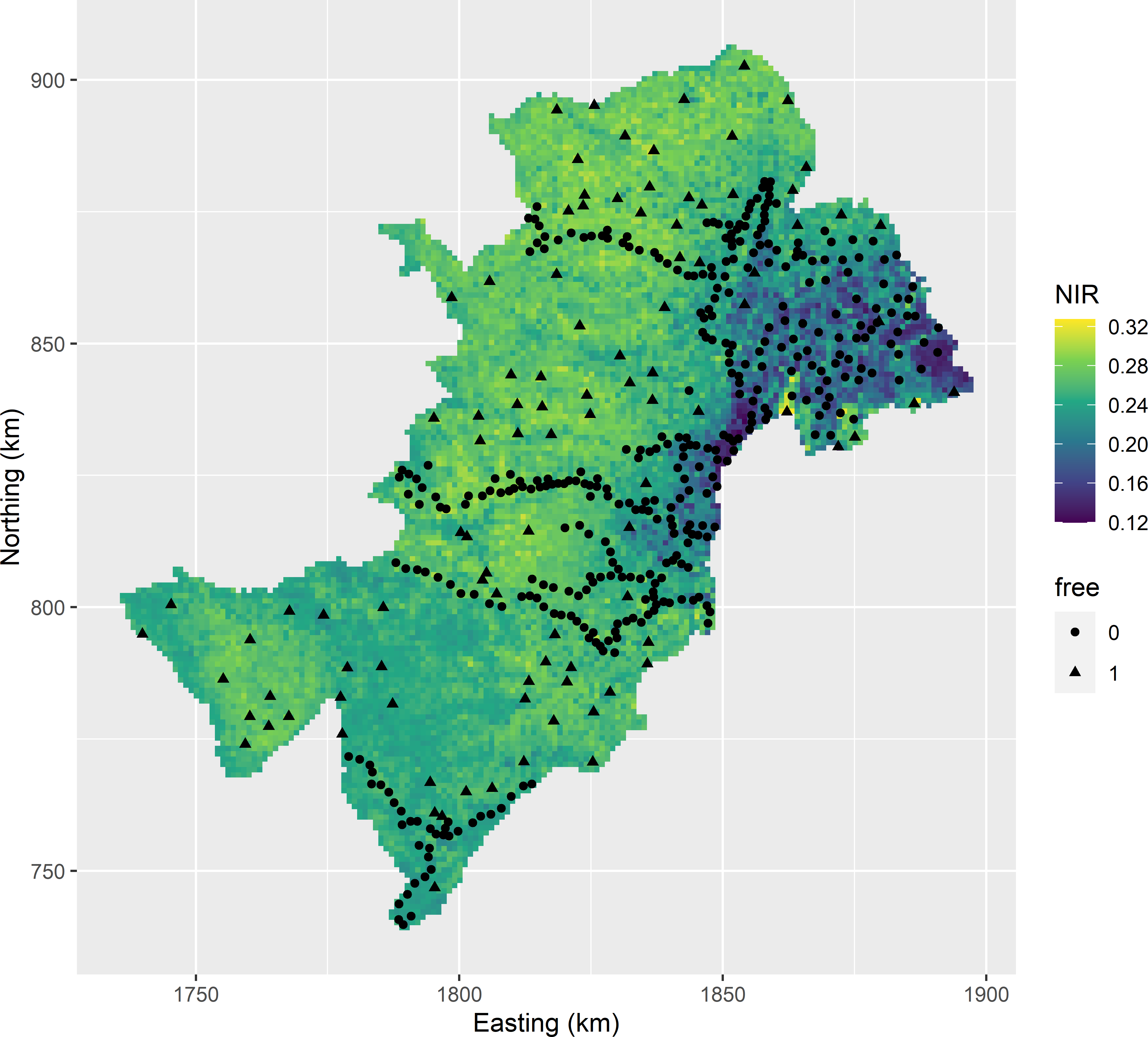
Figure 23.8: Model-based infill sample for KED of the SOM concentration throughout West-Amhara, plotted on a map of one of the covariates. Legacy units have free-value 0; infill units have free-value 1.

The MKV of the optimised sample equals 0.878 (dag kg^-1)², which is somewhat larger than the sill (sum of nugget and partial sill) of the residual semivariogram (Table 22.2). This can be explained by the very small range of the semivariogram, so that ignoring the uncertainty about the model-mean, the kriging variance at nearly all locations in the study area equals the sill. Besides, we are uncertain about the model-mean, explaining that the MKV can be larger than the sill.

References

Akramkhanov, A., D. J. Brus, and D. J. J. Walvoort. 2014. “Geostatistical monitoring of soil salinity in Uzbekistan by repeated EMI surveys.” Geoderma 213: 600–607.

Brus, D. J., J. J. de Gruijter, and J. W. van Groenigen. 2007. “Designing Spatial Coverage Samples Using the k-means Clustering Algorithm.” In Digital Soil Mapping. An Introductory Perspective, edited by P. Lagacherie, A. B. McBratney, and M. Voltz, 183–92. Elsevier.

Brus, D. J., and G. B. M. Heuvelink. 2007. “Optimization of Sample Patterns for Universal Kriging of Environmental Variables.” Geoderma 138 (1–2): 86–95.

Heuvelink, G. B. M., D. J. Brus, and J. J. de Gruijter. 2007. “Optimization of Sample Configurations for Digital Mapping of Soil Properties with Universal Kriging.” In Digital Soil Mapping. An Introductory Perspective, edited by P. Lagacherie, A. B. McBratney, and M. Voltz, 137–51. Elsevier.

Kirkpatrick, S., C. D. Gelatt, and M. P. Vecchi. 1983. “Optimization by Simulated Annealing.” Science 220 (4598): 671–80. https://doi.org/https://doi.org/10.1126/science.220.4598.671.

Pebesma, E. J. 2004. “Multivariable Geostatistics in S: The Gstat Package.” Computers & Geosciences 30 (7): 683–91.

Samuel-Rosa, A. 2019. spsann: Optimization of Sample Configurations using Spatial Simulated Annealing. https://CRAN.R-project.org/package=spsann.

van Groenigen, J. W., G. Pieters, and A. Stein. 2000. “Optimizing Spatial Sampling for Multivariate Contamination in Urban Areas.” Environmetrics 11 (2): 227–44.

van Groenigen, J. W., W. Siderius, and A. Stein. 1999. “Constrained Optimisation of Soil Sampling for Minimisation of the Kriging Variance.” Geoderma 87 (3): 239–59.

van Groenigen, J. W., and A. Stein. 1998. “Constrained Optimization of Spatial Sampling Using Continuous Simulated Annealing.” Journal of Environmental Quality 27 (5): 1078–86.

---

14. At the moment of writing this book, package spsann is not available on CRAN. You can install spsann and its dependency pedometrics with remotes::install_github("samuel-rosa/spsann") and remotes::install_github("samuel-rosa/pedometrics").↩︎