Chapter 5 Systematic random sampling
A simple way of drawing probability samples whose units are spread uniformly over the study area is systematic random sampling (SY), which from a two-dimensional spatial population entails the selection of a regular grid randomly placed on the area. A systematic sample can be selected with function spsample of package sp with argument type = "regular" (Bivand, Pebesma, and Gómez-Rubio 2013). Argument offset is not used, so that the grid is randomly placed on the study area. This is illustrated with Voorst. First, data.frame grdVoorst is converted to SpatialPixelsDataFrame with function gridded.
library(sp)
gridded(grdVoorst) <- ~ s1 + s2
n <- 40
set.seed(777)
mySYsample <- spsample(x = grdVoorst, n = n, type = "regular") %>%
  as("data.frame")
Figure 5.1 shows the randomly selected systematic sample. The shape of the grid is square, and the orientation is East-West (E-W), North-South (N-S). There is no strict need for random selection of the orientation of the grid. Random placement of the grid on the study area suffices for design-based estimation.
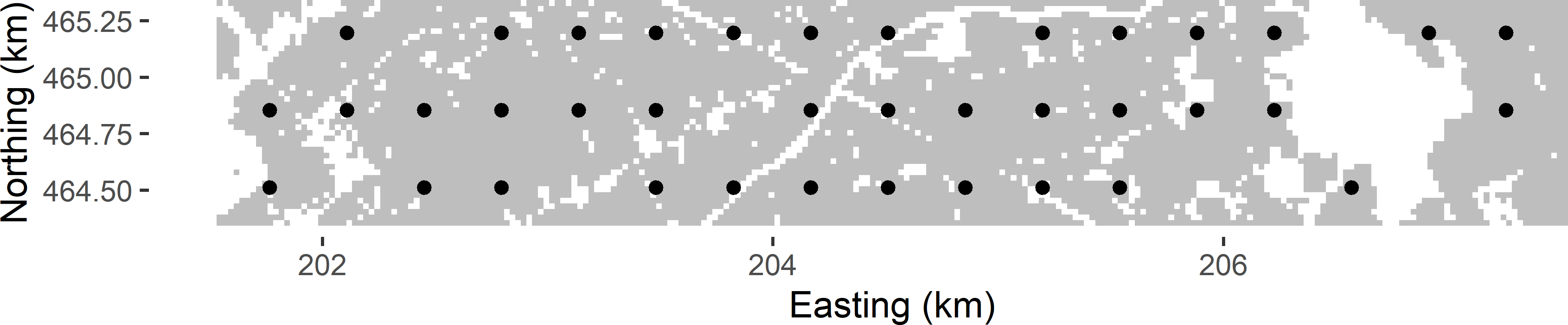
Figure 5.1: Systematic random sample (square grid) from Voorst.
Argument n in function spsample is used to set the sample size. Note that this is the expected sample size, i.e., on average over repeated sampling the sample size is 40. In Figure 5.1 the number of selected sampling points equals 38. Given the expected sample size, the spacing of the square grid can be computed with \(\sqrt{A/n}\), with \(A\) the area of the study area. This area \(A\) can be computed by the total number of cells of the discretisation grid multiplied by the area of a grid cell. Note that the area of the study area is smaller than the number of grid cells in the horizontal direction multiplied by the number of grid cells in the vertical direction multiplied by the grid cell area, as we have non-availables (built-up areas, roads, etc.).
[1] 342.965Instead of argument n we may use argument cell_size to select a grid with a specified spacing. The expected sample size of a square grid can then be computed with \(A/spacing^2\).
The spatial coverage with random grid sampling is better than that with stratified random sampling using compact geographical strata (Section 4.6), even with one sampling unit per geostratum. Consequently, in general systematic random sampling results in more precise estimates of the mean or total.
However, there are also two disadvantages of systematic random sampling compared to geographically stratified random sampling. First, for systematic random sampling, no design-unbiased estimator of the sampling variance exists. Second, the number of sampling units with random grid sampling is not fixed, but varies among randomly drawn samples. We may choose the grid spacing such that on average the number of sampling units equals the required (allowed) number of sampling units, but for the actually drawn sample, this number can be smaller or larger. In Voorst the variation of the sample size is quite large. The approximated sampling distribution, obtained by repeating the sampling 10,000 times, is bimodal (Figure 5.2). The smaller sample sizes are of square grids with only two E-W oriented rows of points instead of three rows.
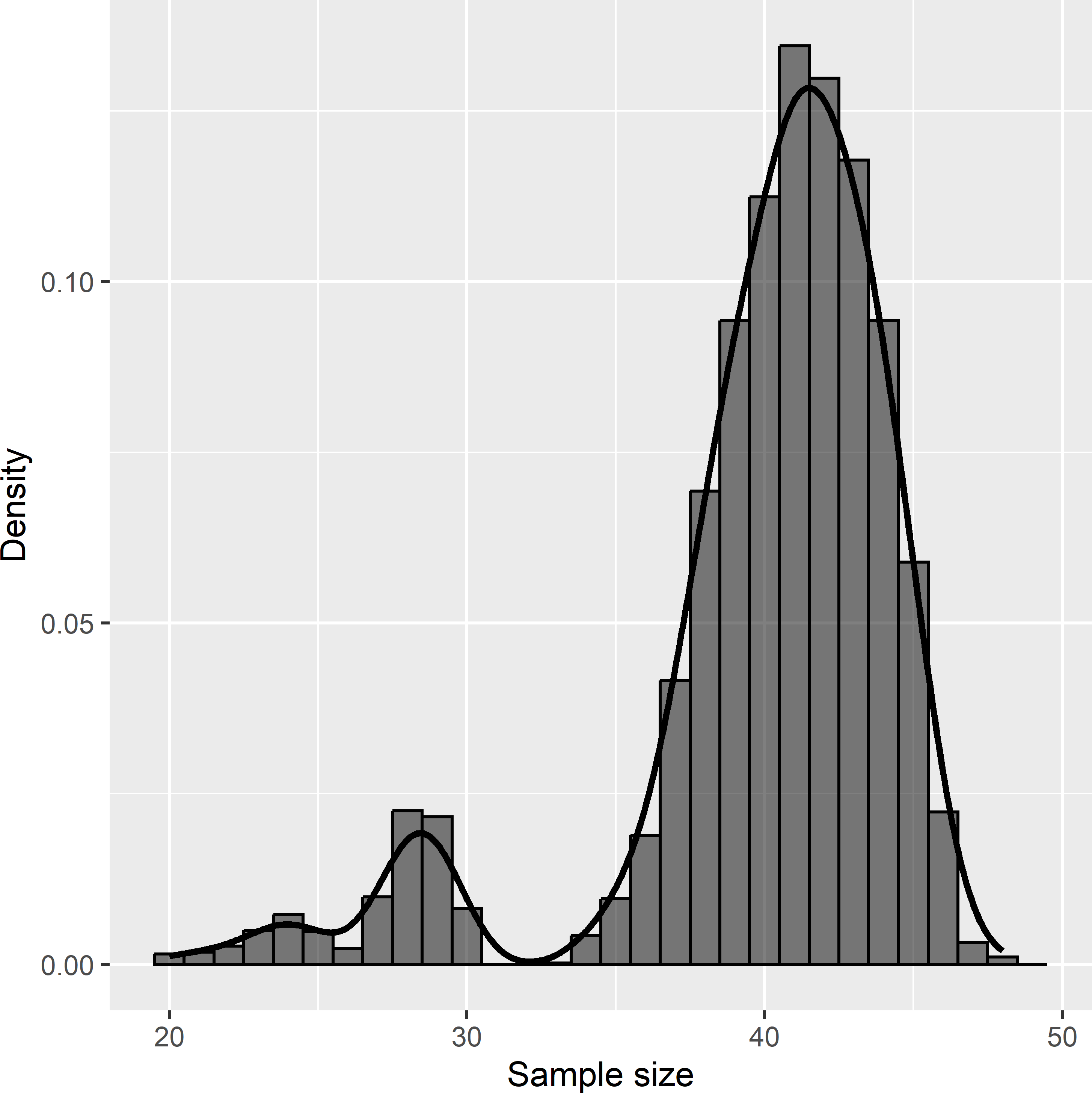
Figure 5.2: Approximated sampling distribution of the sample size of systematic random samples from Voorst. The expected sample size is 40.
A large variation in sample size over repeated selection with the sampling design under study is undesirable and should be avoided when possible. In the case of Voorst, a simple solution is to select a rectangular grid instead of a square grid, with a spacing in the N-S direction that results in a fixed number of E-W oriented rows of sampling points over repeated selection of grids. This is achieved with a N-S spacing equal to the dimension of the study area in N-S direction divided by an integer. The spacing in E-W direction is then adapted so that on average a given number of sampling points is selected. As the N-S dimension of Voorst is 1,000 m, a N-S spacing of 1,000/3 m is chosen, so that the number of E-W oriented rows of sampling points in the systematic sample equals three for any randomly selected rectangular grid.
dy <- 1000 / 3
dx <- A / (n * dy)
mySYsample_rect <- spsample(
  x = grdVoorst, cellsize = c(dx, dy), type = "regular")
The E-W spacing is somewhat larger than the N-S spacing: 352.875 m vs. 333.333 m. The variation in sample size with the random rectangular grid is much smaller than that of the square grid. The sample size now ranges from 33 to 46, whereas with the square grid the range varies from 20 to 48.
   Min. 1st Qu.  Median    Mean 3rd Qu.    Max.
  33.00   38.00   40.00   39.99   42.00   46.00
An alternative shape for the sampling grid is triangular. Triangular grids can be selected with argument type = "hexagonal". The centres of hexagonal sampling grid cells form a triangular grid. The triangular grid was shown to yield most precise estimates of the population mean given the expected sample size (Matérn 1986). Given the spacing of a triangular grid, the expected sample size can be computed by the area \(A\) of the study area divided by the area of hexagonal grid cells with the sampling points at their centres. The area of a hexagon equals \(6\sqrt{3}/4\;r^2\), with \(r\) the radius of the circle circumscribing the hexagon (distance from centre to a corner of the hexagon). So, by choosing a radius of \(\sqrt{A/(6\sqrt{3}/4)\;n}\) the expected sample equals \(n\). The distance between neighbouring points of the triangular grid in the E-W direction, \(dx\), then equals \(r \sqrt{3}\). The N-S distance equals \(\sqrt{3}/2 \; dx\).
Function spsample does not work properly in combination with argument type = "hexagonal". Over repeated sampling, the average sample size is not equal to the chosen sample size passed to function spsample with argument n. The same problem remains when using argument cellsize.
   Min. 1st Qu.  Median    Mean 3rd Qu.    Max.
  18.00   23.00   26.00   28.39   35.00   41.00
The following code can be used for random selection of triangular grids.
SY_triangular <- function(dx, grd) {
  dy <- sqrt(3) / 2 * dx
  #randomly select offset
  offset_x <- runif(1, min = 0, max = dx)
  offset_y <- runif(1, min = 0, max = dy)
  #compute x-coordinates of 1 row and y-coordinates of 1 column
  bbox <- bbox(grd)
  nx <- ceiling((bbox[1, 2] - bbox[1, 1]) / dx)
  ny <- ceiling((bbox[2, 2] - bbox[2, 1]) / dy)
  x <- (-1:nx) * dx + offset_x
  y <- (0:ny) * dy + offset_y
  #compute coordinates of rectangular grid
  xy <- expand.grid(x, y)
  names(xy) <- c("x", "y")
  #shift points of even rows in horizontal direction
  units <- which(xy$y %in% y[seq(from = 2, to = ny, by = 2)])
  xy$x[units] <- xy$x[units] + dx / 2
  #add coordinates of origin
  xy$x <- xy$x + bbox[1, 1]
  xy$y <- xy$y + bbox[2, 1]
  #overlay with grid
  coordinates(xy) <- ~ x + y
  mysample <- data.frame(coordinates(xy), over(xy, grd))
  #delete points with NA
  mysample <- mysample[!is.na(mysample[, 3]), ]
}
set.seed(314)
mySYsample_tri <- SY_triangular(dx = dx, grd = grdVoorst)
Figure 5.3 shows a triangular grid, selected randomly from Voorst with an expected sample size of 40. The selected triangular grid has 42 points.
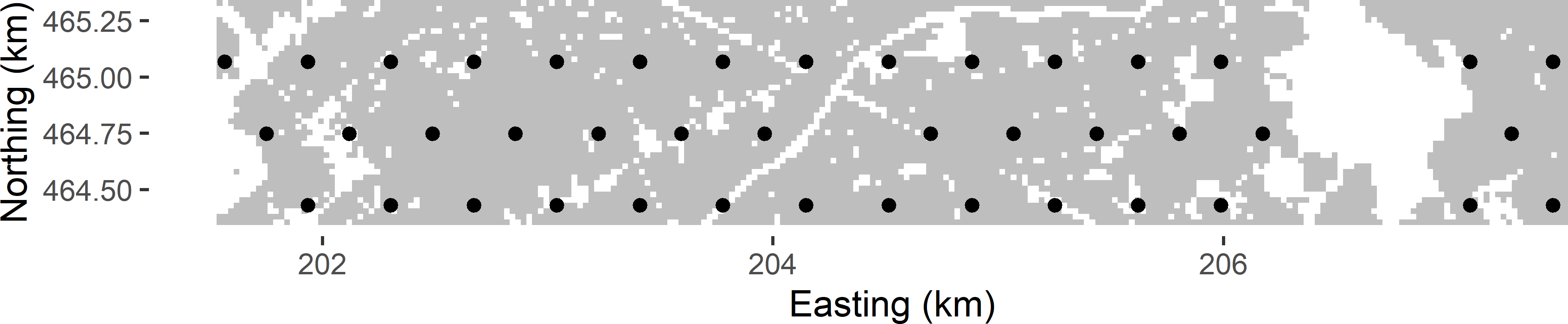
Figure 5.3: Systematic random sample (triangular grid) from Voorst.
5.1 Estimation of population parameters
With systematic random sampling, all units have the same inclusion probability, equal to \(E[n]/N\), with \(E[n]\) the expected sample size. Consequently, the population total can be estimated by
\[\begin{equation} \hat{t}(z)=\sum_{k \in \mathcal{S}}\frac{z_k}{\pi_k} = N \sum_{k \in \mathcal{S}}\frac{z_k}{E[n]} \;. \tag{5.1} \end{equation}\]
The population mean can be estimated by dividing this \(\pi\) estimator of the population total by the population size:
\[\begin{equation} \hat{\bar{z}}=\sum_{k \in \mathcal{S}}\frac{z_k}{E[n]} \;. \tag{5.2} \end{equation}\]
In this \(\pi\) estimator of the population mean the sample sum of the observations is not divided by the number of selected units \(n\), but by the expected number of units \(E[n]\).
An alternative estimator is obtained by dividing the \(\pi\) estimator of the population total by the \(\pi\) estimator of the population size:
\[\begin{equation} \hat{N}=\sum_{k \in \mathcal{S}}\frac{1}{\pi_k} = n \frac{N}{E[n]} \;. \tag{5.3} \end{equation}\]
This yields the ratio estimator of the population mean:
\[\begin{equation} \hat{\bar{z}}_{\text{ratio}}=\frac{\hat{t}(z)}{\hat{N}} = \frac{1}{n}\sum_{k \in \mathcal{S}}z_k \;. \tag{5.4} \end{equation}\]
So, the ratio estimator of the population total is equal to the unweighted sample mean. In general, the variance of this ratio estimator is smaller than that of the \(\pi\) estimator. On the other hand the \(\pi\) estimator is design-unbiased, whereas the ratio estimator is not, although its bias can be negligibly small. Only in the very special case where the sample size with systematic random sampling is fixed, the two estimators are equivalent.
Recall that for Voorst we have exhaustive knowledge of the study variable \(z\): values of the soil organic matter (SOM) concentration were simulated for all grid cells. To determine the \(z\)-values at the selected sampling points, an overlay of the systematic random sample and the SpatialPixelsDataFrame is made, using function over of package sp.
res <- over(mySYsample, grdVoorst)
mySYsample <- as(mySYsample, "data.frame")
mySYsample$z <- res$z
mz_HT <- sum(mySYsample$z) / n
mz_ratio <- mean(mySYsample$z)
Using the systematic random sample of Figure 5.1, the \(\pi\) estimated mean SOM concentration equals 69.8 g kg-1, the ratio estimate equals 73.5 g kg-1. The ratio estimate is larger than the \(\pi\) estimate, because the size of the selected sample is two units smaller (38) than the expected sample size (40).
5.2 Approximating the sampling variance of the estimator of the mean
An unbiased estimator of the sampling variance of the estimator of the mean is not available. A simple, often applied procedure is to calculate the sampling variance as if the sample were a simple random sample (Equation (3.10) or (3.11)). In general, this procedure overestimates the sampling variance, so that we are on the safe side.
The approximated variance equals 50.3 (g kg-1)2.
Alternatively, the sampling variance can be estimated by treating the systematic random sample as if it were a stratified simple random sample (Equation (4.4)). The sampling units are clustered on the basis of their spatial coordinates into \(H=n/2\) clusters (\(n\) even) or \(H=(n-1)/2\) clusters (\(n\) odd). In the next code chunk, a simple k-means function is defined to cluster the sampling units of the grid into equal-sized clusters. Arguments s1 and s2 are the spatial coordinates of the sampling units, k is the number of clusters. First, in this function the ids of equal-sized clusters are randomly assigned to the sampling units on the nodes of the sampling grid (initial clustering). Next, the centres of the clusters, i.e., the means of the spatial coordinates of the clusters (initial cluster centres), are computed. There are two for-loops. In the inner loop it is determined whether the cluster id of the unit selected in the outer loop should be swopped with the cluster id of the next unit. If both units have the same cluster id the next unit is selected, until a unit of a different cluster is found. The cluster ids of the two units are swopped when the sum of the squared distances of the two units to their corresponding cluster centres is reduced. When the cluster ids are swopped, the centres are recomputed. The two loops are repeated until no swops are made anymore.
.kmeans_equal_size <- function(s1, s2, k) {
  n <- length(s1)
  cluster_id <- rep(1:k, times = ceiling(n / k))
  cluster_id <- cluster_id[1:n]
  cluster_id <- cluster_id[sample(n, size = n)]
  s1_c <- tapply(s1, INDEX = cluster_id, FUN = mean)
  s2_c <- tapply(s2, INDEX = cluster_id, FUN = mean)
  repeat {
    n_swop <- 0
    for (i in 1:(n - 1)) {
      ci <- cluster_id[i]
      for (j in (i + 1):n) {
        cj <- cluster_id[j]
        if (ci == cj) {
          next
          }
        d1 <- (s1[i] - s1_c[ci])^2 + (s2[i] - s2_c[ci])^2 +
          (s1[j] - s1_c[cj])^2 + (s2[j] - s2_c[cj])^2
        d2 <- (s1[i] - s1_c[cj])^2 + (s2[i] - s2_c[cj])^2 +
          (s1[j] - s1_c[ci])^2 + (s2[j] - s2_c[ci])^2
        if (d1 > d2) {
          #swop cluster ids and recompute cluster centres
          cluster_id[i] <- cj; cluster_id[j] <- ci
          s1_c <- tapply(s1, cluster_id, mean)
          s2_c <- tapply(s2, cluster_id, mean)
          n_swop <- n_swop + 1
          break
        }
      }
    }
    if (n_swop == 0) {
      break
      }
  }
  D <- fields::rdist(x1 = cbind(s1_c, s2_c), x2 = cbind(s1, s2))
  dmin <- apply(D, MARGIN = 2, FUN = min)
  MSSD <- mean(dmin^2)
  list(clusters = cluster_id, MSSD = MSSD)
}
The clustering is repeated 100 times (ntry = 100). The clustering with the smallest mean of the squared distances of the sampling units to their cluster centres (mean squared shortest distance, MSSD) is selected.
kmeans_equal_size <- function(s1, s2, k, ntry) {
  res_opt <- NULL
  MSSD_min <- Inf
  for (i in 1:ntry) {
      res <- .kmeans_equal_size(s1, s2, k)
      if (res$MSSD < MSSD_min) {
        MSSD_min <- res$MSSD
        res_opt <- res
      }
  }
  res_opt
}
n <- nrow(mySYsample); k <- floor(n / 2)
set.seed(314)
res <- kmeans_equal_size(s1 = mySYsample$x1 / 1000, s2 = mySYsample$x2 / 1000,
  k = k, ntry = 100)
mySYsample$cluster <- res$clusters
Figure 5.4 shows the clustering of the systematic random sample of Figure 5.1. The two or three sampling units of a cluster are treated as a simple random sample from a stratum, and the variance estimator for stratified random sampling is used. The weights are computed by \(w_h=n_h/n\). With \(n\) even the stratum weight is \(1/H\) for all strata. For more details on variance estimation with stratified simple random sampling, refer to Section 4.1.
S2z_h <- tapply(mySYsample$z, INDEX = mySYsample$cluster, FUN = var)
nh <- tapply(mySYsample$z, INDEX = mySYsample$cluster, FUN = length)
v_mz_h <- S2z_h / nh
w_h <- nh / sum(nh)
av_STSI_mz <- sum(w_h^2 * v_mz_h)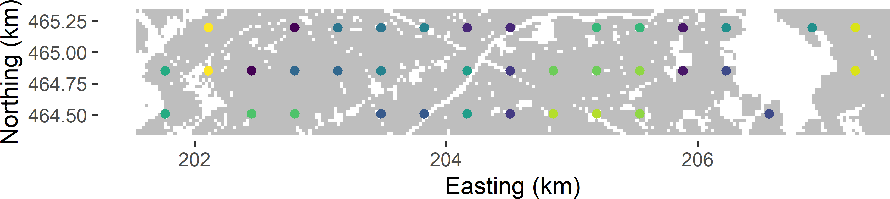
Figure 5.4: Clustering of grid points for approximating the variance of the ratio estimator of the mean SOM concentration in Voorst.
This method yields an approximated variance of 51.2 (g kg-1)2, which is for the selected triangular grid slightly larger than the simple random sample approximation. Hereafter, we will see that on average the stratified simple random sample approximation of the variance is smaller than the simple random sample approximation. For an individual sample, the reverse can be true.
A similar approach for approximating the variance was proposed by Matérn (Matérn 1947) a long time ago. In this approach the variance is approximated by computing the squared difference of two local means. A local mean is computed by linear interpolation of the observations at the two nodes on the diagonal of a square sampling grid cell. The four corners of a sampling grid cell serve as a group. Every sampling grid node belongs to four groups, and so the observation at a sampling grid node is used four times in computing a local mean. Near the edges of the study area, we have incomplete groups: one, two, or even three observations are missing. To compute a squared difference, these missing values are replaced by the sample mean. This results in as many squared differences as we have groups. Note that the number of groups is larger than the sample size. The squared differences are computed by
\[\begin{equation} \begin{split} d^2_{r,s} & = \left(\frac{z_{r,s}+z_{r+1,s+1}}{2}-\frac{z_{r+1,s}+z_{r,s+1}}{2}\right)^2 \\ & =\frac{(z_{r,s}-z_{r+1,s}-z_{r,s+1}+z_{r+1,s+1})^2}{4}\;, \end{split} \tag{5.5} \end{equation}\]
with \(r = 0,1, \dots ,R\) an index for the column number and \(s=0,1, \dots, S\) an index for the row number of the extended grid. The variance of the estimator of the mean (sample mean) is then approximated by the sum of the squared differences divided by the squared sample size:
\[\begin{equation} \widehat{V}(\bar{z}_{\mathcal{S}}) = \frac{\sum_{g=1}^G d^2_g}{n^2}\;, \tag{5.6} \end{equation}\]
with \(d^2_g\) the squared difference of group unit \(g\), and \(G\) the total number of groups.
To approximate the variance with Matérn’s method, a function is defined.
matern <- function(s) {
  g_11 <- within(s, {gr <- i; gs <- j; z11 <- z})[, c("gr", "gs", "z11")]
  g_12 <- within(s, {gr <- i; gs <- j - 1; z12 <- z})[, c("gr", "gs", "z12")]
  g_21 <- within(s, {gr <- i - 1; gs <- j; z21 <- z})[, c("gr", "gs", "z21")]
  g_22 <- within(s, {gr <- i - 1; gs <- j - 1; z22 <- z})[, c("gr", "gs", "z22")]
  g <- Reduce(function(x, y) merge(x = x, y = y, by = c("gr", "gs"), all = TRUE),
              list(g_11, g_12, g_21, g_22))
  g[is.na(g)] <- mean(s$z)
  g <- within(g, T <- (z11 - z12 - z21 + z22)^2 / 4)
  sum(g$T) / ((nrow(s))^2)
}
Before using this function the data frame with the sample data must be extended with two variables: an index \(i\) for the column number and an index \(j\) for the row number of the square grid.
mySYsample <- mySYsample %>%
  mutate(
    i = round((x1 - min(x1)) / spacing),
    j = round((x2 - min(x2)) / spacing))
matern(mySYsample)
[1] 41.63163Figure 5.5 shows the approximated sampling distributions of estimators of the mean SOM concentration for systematic random sampling, using a randomly placed square grid with fixed orientation and an expected sample size of 40, and for simple random sampling, obtained by repeating the random sampling with each design and estimation 10,000 times. To estimate the population mean from the systematic random samples, both the \(\pi\) estimator and the ratio estimator are used.
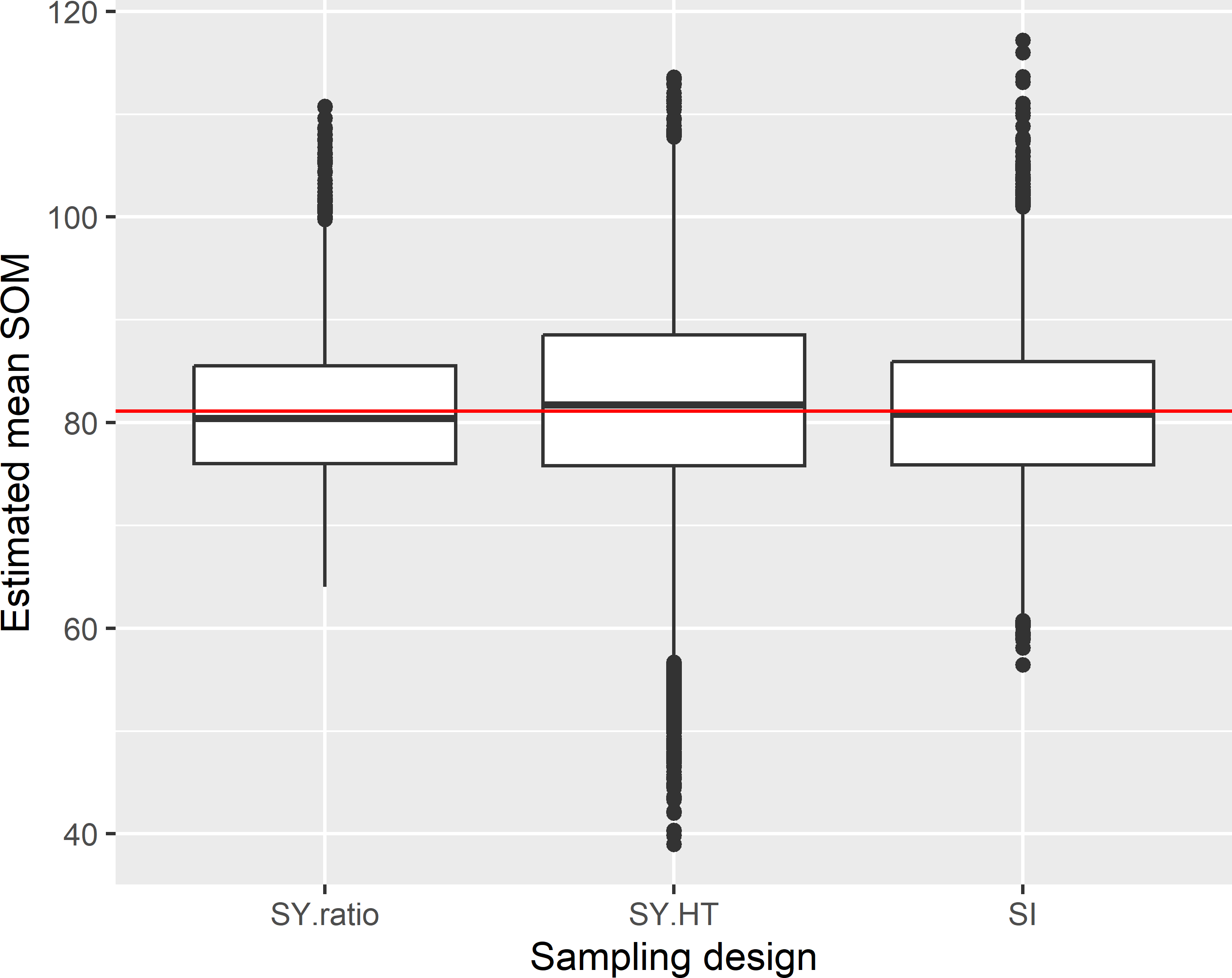
Figure 5.5: Approximated sampling distribution of estimators of the mean SOM concentration (g kg-1) in Voorst, for systematic random sampling (square grid) and simple random sampling and an expected sample size of 40. With systematic random sampling, both the \(\pi\) estimator (SY.HT) and the ratio estimator (SY.ratio) are used in estimation.
The boxplots of the estimated means indicate that systematic random sampling in combination with the ratio estimator is more precise than simple random sampling. The variance of the 10,000 ratio estimates equals 49.0 (g kg-1)2, whereas for simple random sampling this variance equals 55.4 (g kg-1)2. Systematic random sampling in combination with the \(\pi\) estimator performs very poorly: the variance equals 142.6 (g kg-1)2. This can be explained by the strong variation in sample size (Figure 5.2), which is not accounted for in the \(\pi\) estimator.
The mean of the 10,000 ratio estimates is 81.2 g kg-1, which is about equal to the population mean 81.1 g kg-1, showing that in this case the design-bias of the ratio estimator is negligibly small indeed.
The average of the 10,000 approximated variances treating the systematic sample as a simple random sample equals 56.4 (g kg-1)2. This is larger than the variance of the ratio estimator (49.0 (g kg-1)2). The stratified simple random sample approximation of the variance somewhat underestimates the variance: the mean of this variance approximation equals 47.1 (g kg-1)2. Also with Matérn’s method, the variance is underestimated in this case: the mean of the 10,000 variances equals 45.6 (g kg-1)2. Figure 5.6 shows boxplots of the approximated standard error of the ratio estimator of the population mean. The horizontal red line is at the standard deviation of the 10,000 ratio estimates of the population mean. Differences between the three approximation methods are small in this case.
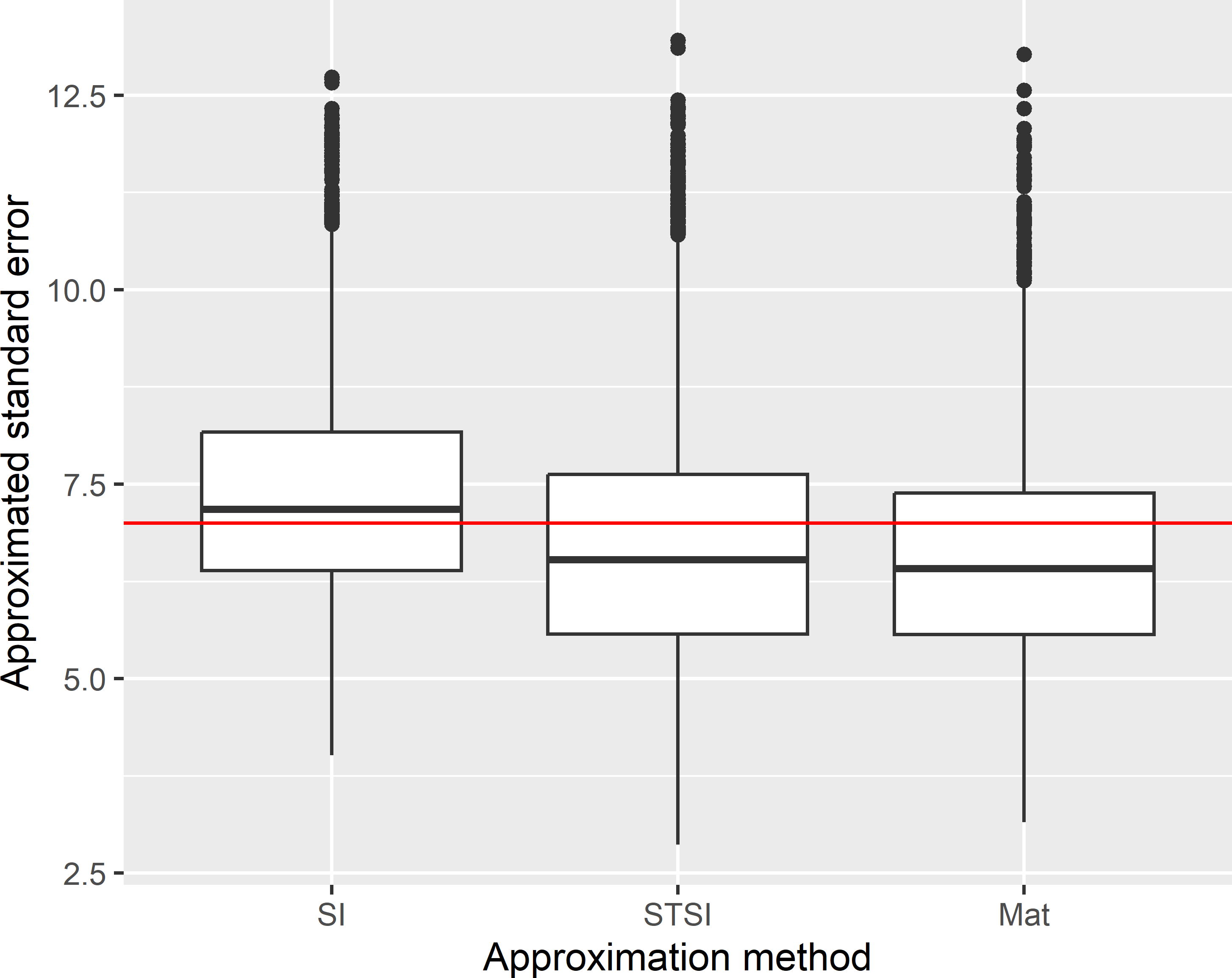
Figure 5.6: Sampling distribution of the approximated standard error of the ratio estimator of the mean SOM concentration (g kg-1) in Voorst, with systematic random sampling (square grid) and an expected sample size of 40. Approximations are obtained by treating the systematic sample as a simple random sample (SI) or a stratified simple random sample (STSI), and with Matérn’s method (Mat).
The variance of the 10,000 ratio estimates of the population mean with the triangular grid and an expected sample size of 40 equals 46.9 (g kg-1)2. Treating the triangular grid as a simple random sample strongly overestimates the variance: the average approximated variance equals 60.1 (g kg-1)2. The stratified simple random sample approximation performs much better in this case: the average of the 10,000 approximated variances equals 46.8 (g kg-1)2. Matérn’s method cannot be used to approximate the variance with a triangular grid.
The approximated variance for this clustering equals 90.3.
Brus and Saby (2016) compared various variance approximations for systematic random sampling, among which model-based prediction of the variance, using a semivariogram that is estimated from the systematic sample, see Chapter 13.
Exercises
- One solution to the problem of variance estimation with systematic random sampling is to select multiple systematic random samples independently from each other. So, for instance, instead of one systematic random sample with an expected sample size of 40, we may select two systematic random samples with an expected size of 20.
- Write an R script to select two systematic random samples (random square grids) both with an expected size of 20 from Voorst.
- Use each sample to estimate the population mean, so that you obtain two estimated means. Overlay the points of each sample with
grdVoorst, using functionoverand extract the \(z\)-values. - Use the two estimated means to estimate the sampling variance of the estimator of the mean for systematic random sampling with an expected sample size of 20.
- Use the two estimated means to compute a single, final estimate of the population mean, as estimated from two systematic random samples, each with an expected sample size of 20.
- Estimate the sampling variance of the final estimate of the population mean.
- Do you like this solution? What about the variance of the estimator of the mean, obtained by selecting two systematic random samples of half the expected size, as compared with the variance of the estimator of the mean, obtained with a single systematic random sample? Hint: plot the two random square grids. What do you think of the spatial coverage of the two samples?