Chapter 17 Regular grid and spatial coverage sampling

This chapter describes and illustrates two sampling designs by which the sampling locations are evenly spread throughout the study area: regular grid sampling and spatial coverage sampling. In a final section, the spatial coverage sampling design is used to fill in the empty spaces of an existing sample.

17.1 Regular grid sampling

Sampling on a regular grid is an attractive option for mapping because of its simplicity. The data collected on the grid nodes are not used for design-based estimation of the population mean or total. For this reason, the grid need not be placed randomly on the study area as in systematic random sampling (Chapter 5). The grid can be located such that the grid nodes optimally cover the study area in the sense of the average distance of the nodes of a fine discretisation grid to the nearest node of the sampling grid. Commonly used grid configurations are square and triangular. If the grid data are used in kriging (Chapter 21), the optimal configuration depends, among others, on the semivariogram model. If the study variable shows moderate to strong spatial autocorrelation (see Section 21.1), triangular grids outperform square grids.

Besides the shape of the sampling grid cells, we must decide on the grid spacing. The grid spacing determines the number of sampling units in the study area, i.e., the sample size. There are two options to decide on this spacing, either starting from the available budget or from a requirement on the quality of the map. The latter is explained in Chapter 22, as this requires a model of the spatial variation, and as a consequence this is an example of model-based sampling. Starting from the available budget and an estimate of the costs per sampling unit, we first compute the affordable sample size. Then we may derive from this number the grid spacing. For square grids, the grid spacing in meters is calculated as \(\sqrt{A/n}\), where \(A\) is the area in m² and \(n\) is the number of sampling units (sample size).

Grids can be selected with function spsample of package sp (E. J. Pebesma and Bivand 2005). Argument offset is used to select a grid non-randomly. Either a sample size can be specified, using argument n, or a grid spacing, using argument cellsize. In the next code chunk, a square grid is selected with a spacing of 200 m.

library(sp)
gridded(grdVoorst) <- ~ s1 + s2
mysample <- spsample(
  x = grdVoorst, type = "regular", cellsize = c(200, 200),
  offset = c(0.5, 0.5)) %>% as("data.frame")

Figure 17.1 shows the selected square grid.

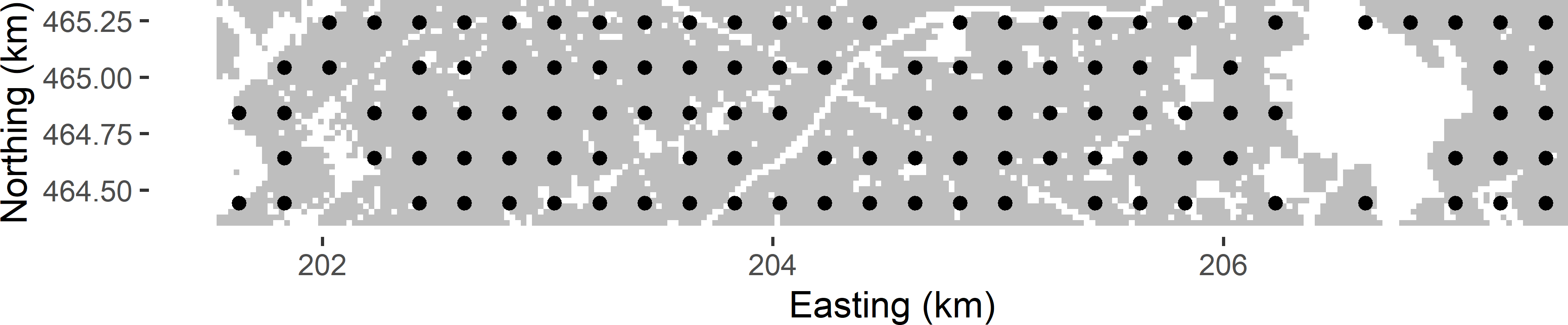
Figure 17.1: Non-random square grid sample with a grid spacing of 200 m from Voorst.

The number of grid points in this example equals 115. Nodes of the square grid in parts of the area not belonging to the population of interest, such as built-up areas and roads, are discarded by spsample (these nodes are not included in the sampling frame file grdVoorst). As a consequence, there are some undersampled areas, for instance in the middle of the study area where two roads cross. If we use the square grid in spatial interpolation, e.g., by ordinary kriging, we are more uncertain about the predictions in these undersampled areas than in areas where the grid is complete. The next section will show how this local undersampling can be avoided.

Exercises

1. Write an R script to select a square grid of size 100 from West-Amhara in Ethiopia. Use grdAmhara of package sswr as a sampling frame. Use a fixed starting point of the grid, i.e., do not select the grid randomly.
   • Compute the number of selected grid points. How comes it is not exactly equal to 100?
   • Select a square grid with a spacing of 10.2 km, and compute the sample size.
   • Write a for-loop to select 200 times a square grid of, on average, 100 points with random starting point. Set a seed so that the result can be reproduced. Determine for each randomly selected grid the number of selected grid points, and save this in a numeric. Compute summary statistics of the sample size, and plot a histogram.
   • Select a square grid of exactly 100 points.

17.2 Spatial coverage sampling

Local undersampling with regular grids can be avoided by relaxing the constraint that the sampling units are restricted to the nodes of a regular grid. This is what is done in spatial coverage sampling or, in case of a sample that is added to an existing sample, in spatial infill sampling. Spatial coverage and infill samples cover the area or fill in the empty space as uniformly as possible. The sampling units are obtained by minimising a criterion that is defined in terms of the geographic distances between the nodes of a fine discretisation grid and the sampling units. Brus, de Gruijter, and van Groenigen (2007) proposed to minimise the mean of the squared distances of the grid nodes to their nearest sampling unit (mean squared shortest distance, MSSD):

\[\begin{equation} MSSD=\frac{1}{N}\sum_{k=1}^{N}\min_{j}\left(D_{kj}^{2}\right) \;, \tag{17.1} \end{equation}\]

where \(N\) is the total number of nodes of the discretisation grid and \(D_{kj}\) is the distance between the \(k\)th grid node and the \(j\)th sampling point. This distance measure can be minimised by the k-means algorithm, which is a numerical, iterative procedure. Figure 17.2 illustrates the selection of a spatial coverage sample of four points from a square. In this simple example the optimal spatial coverage sample is known, being the centres of the four subsquares of equal size. A simple random sample of four points serves as the initial solution. Each raster cell is then assigned to the closest sampling point. This is the initial clustering. In the next iteration, the centres of the initial clusters are computed. Next, the raster cells are reassigned to the closest new centres. This continues until there is no change anymore. In this case only nine iterations are needed, where an iteration consists of computing the clusters by assigning the raster cells to the nearest centre (sampling unit), followed by computing the centres of these clusters. Figure 17.2 shows the first, second, and ninth iterations.

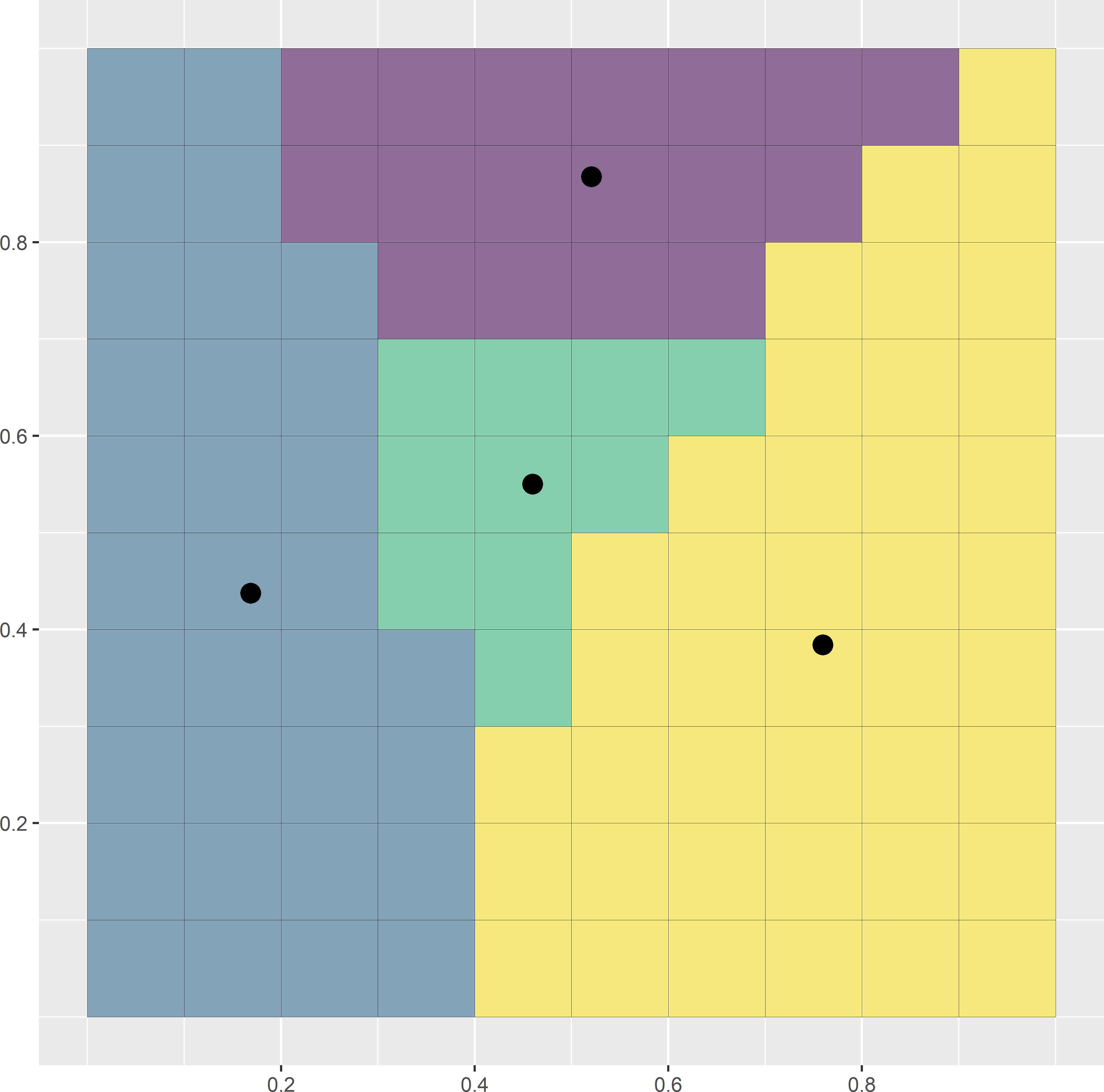
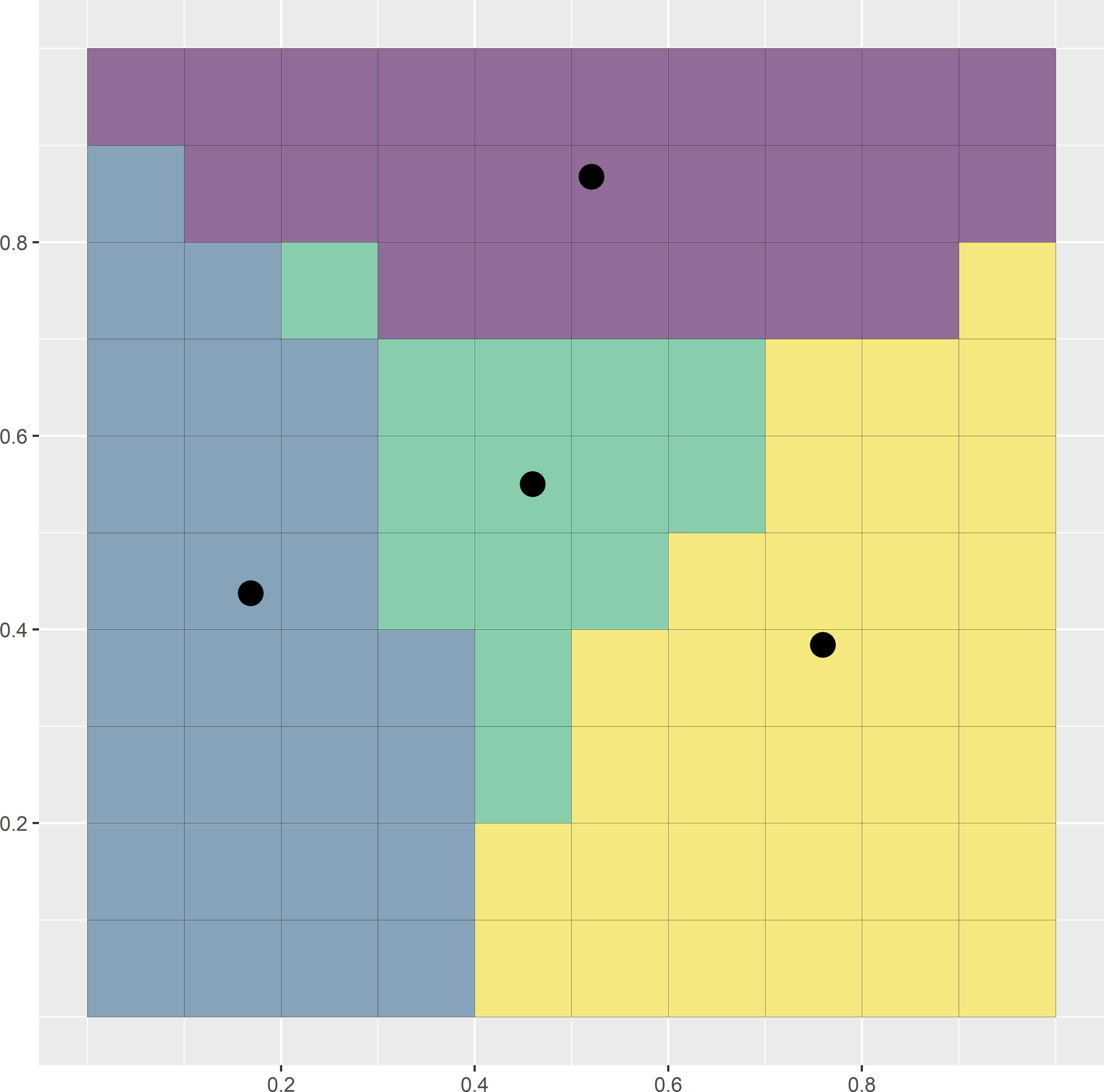
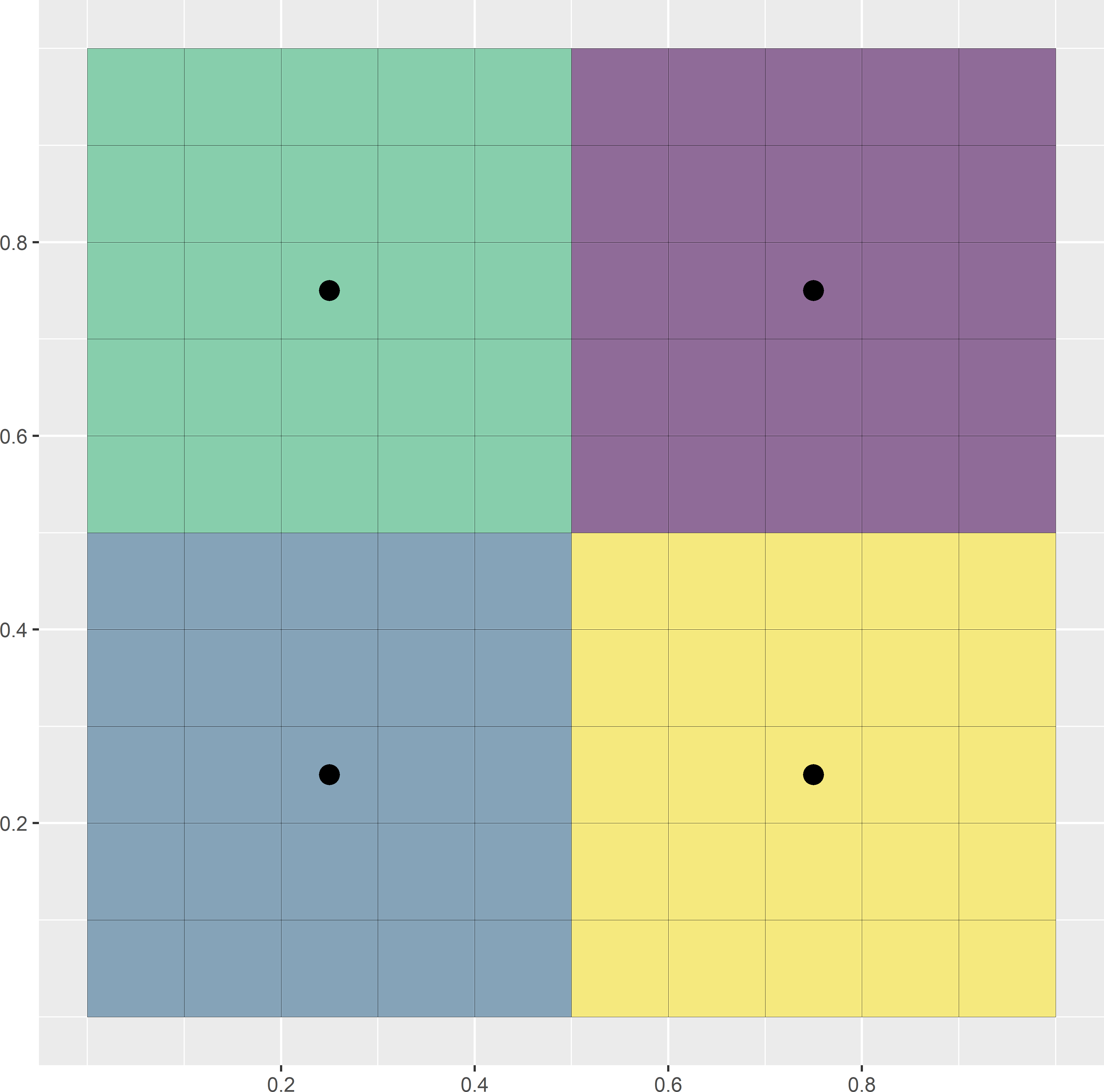
Figure 17.2: First, second, and ninth iterations of the k-means algorithm to select a spatial coverage sample of four points from a square. Iterations are in rows from top to bottom. In the left column of subfigures, the clusters are computed by assigning the raster cells to the nearest centre. In the right column of subfigures, the centres of the clusters are computed.

The same algorithm was used in Chapter 4 to construct compact geographical strata (briefly referred to as geostrata) for stratified random sampling. The clusters serve as strata. In stratified random sampling, one or more sampling units are selected randomly from each geostratum. However, for mapping purposes probability sampling is not required, so the random selection of a unit within each stratum is not needed. With random selection, the spatial coverage is suboptimal. Here, the centres of the final clusters (geostrata) are used as sampling points. This improves the spatial coverage compared to stratified random sampling.

In probability sampling, we may want to have strata of equal area (clusters of equal size) so that the sampling design becomes self-weighting. For mapping, equally sized clusters are not recommended, as this may lead to samples with suboptimal spatial coverage.

In Figure 17.2 the clusters are of equal size, but this is an artefact. Equally sized clusters are not guaranteed by the illustrated k-means algorithm. Clustering the raster cells of a square into four clusters is a very special case. In other cases, the clusters computed with the k-means algorithm described above might have unequal sizes. In package spcosa also a different k-means algorithm is implemented, using swops, enforcing compact clusters of equal size.

Spatial coverage samples can be computed with package spcosa (D. J. J. Walvoort, Brus, and Gruijter 2010), using functions stratify and spsample, see code chunk below. Argument nTry of function stratify specifies the number of initial stratifications in k-means clustering. Note that function spsample of package spcosa without optional argument n selects non-randomly one point in each cluster, being the centre. Figure 17.3 shows a spatial coverage sample of the same size as the regular grid in study area Voorst (Figure 17.1). Note that the undersampled area in the centre of the study area is now covered by a sampling point.

library(spcosa)
n <- 115
set.seed(314)
gridded(grdVoorst) <- ~ s1 + s2
mystrata <- spcosa::stratify(
  grdVoorst, nStrata = n, equalArea = FALSE, nTry = 10)
mysample <- spsample(mystrata) %>% as("data.frame")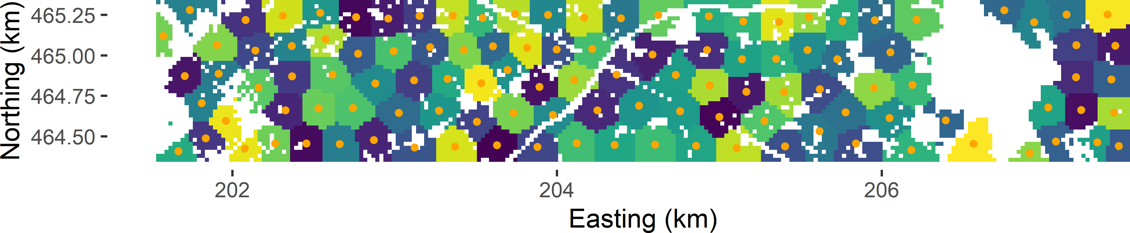

Figure 17.3: Spatial coverage sample from Voorst.

If the clusters need not be of equal size, we may also use function kmeans of the stats package, using the spatial coordinates as clustering variables. This requires less computing time, especially with large data sets.

grdVoorst <- as_tibble(grdVoorst)
mystrata_kmeans <- kmeans(
  grdVoorst[, c("s1", "s2")], centers = n, iter.max = 10000, nstart = 10)
mysample_kmeans <- mystrata_kmeans$centers %>% data.frame()

When function kmeans is used to compute the spatial coverage sample, there is no guarantee that the computed centres of the clusters, used as sampling points, are inside the study area. In Figure 17.4 there are eight such centres.

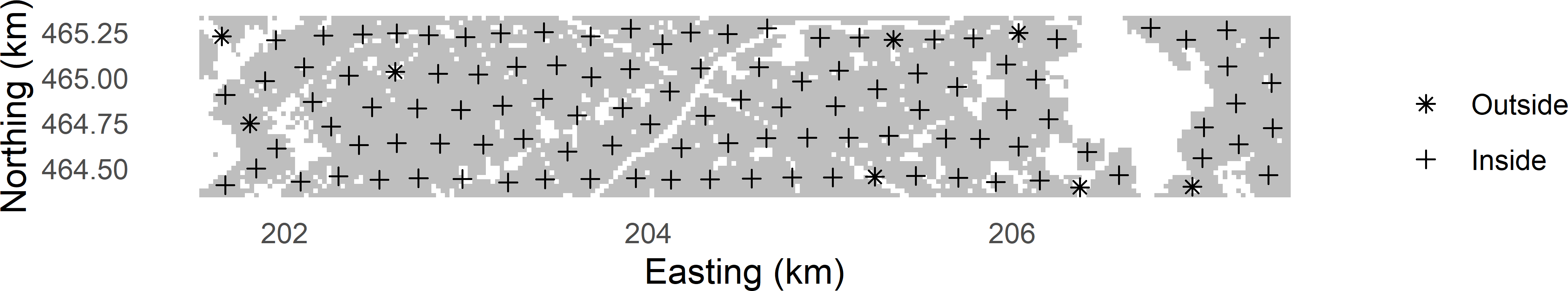
Figure 17.4: Centres of spatial clusters computed with function kmeans.

This problem can easily be solved by selecting points inside the study area closest to the centres that are outside the study area. Function rdist of package fields is used to compute a matrix with distances between the centres outside the study area and the nodes of the discretisation grid. Then function apply is used with argument FUN = which.min to compute the discretisation nodes closest to the centres outside the study area. A similar procedure is implemented in function spsample of package spcosa when the centres of the clusters are selected as sampling points (so, when argument n of function spsample is not used).

library(fields)
gridded(grdVoorst) <- ~ s1 + s2
coordinates(mysample_kmeans) <- ~ s1 + s2
res <- over(mysample_kmeans, grdVoorst)
inside <- as.factor(!is.na(res$z))
units_out <- which(inside == FALSE)
grdVoorst <- as_tibble(grdVoorst)
mysample_kmeans <- as_tibble(mysample_kmeans)
D <- fields::rdist(x1 = mysample_kmeans[units_out, ],
  x2 = grdVoorst[, c("s1", "s2")])
units_close <- apply(D, MARGIN = 1, FUN = which.min)
mysample_kmeans[units_out, ] <- grdVoorst[units_close, c("s1", "s2")]

Exercises

2. In forestry and vegetation surveys, square and circular plots are often used as sampling units, for instance, 2 m squares or circles with a diameter of 2 m. To study the relation between the vegetation and the soil, soil samples must be collected from the vegetation plots. Suppose we want to collect four soil samples from a square plot. Where would you locate the four sampling points, so that they optimally cover the plot?
   
3. Suppose we are also interested in the accuracy of the estimated plot means of the soil properties, not just the means. In that case, the soil samples should not be bulked into a composite sample, but analysed separately. How would you select the sampling points in this case?
   
4. For circular vegetation plots, it is less clear where the sampling points with smallest MSSD are (Equation (17.1)). Write an R script to compute a spatial coverage sample of five points from a circular plot discretised by the nodes of a fine square grid. Use argument equalArea = FALSE. Check the size (number of raster cells) of the strata. Repeat this for six sampling points.
   
5. Consider the case of six strata. The strata are not of equal size. If the soil samples are bulked into a composite sample, the measurement on this single sample is a biased estimator of the plot mean. How can this bias be avoided?

17.3 Spatial infill sampling

If georeferenced data are available that can be used for mapping the study variable, but we need more data for mapping, it is attractive to account for these existing sampling units when selecting the additional units. The aim now is to fill in the empty spaces, i.e., the parts of the study area not covered by the existing sampling units. This is referred to as spatial infill sampling. Existing sampling units can easily be accommodated in the k-means algorithm, using them as fixed cluster centres.

Figure 17.5 shows a spatial infill sample for West-Amhara. A large set of legacy data on soil organic matter (SOM) in mass percentage (dag kg^-1) is available, but these data come from strongly spatially clustered units along roads (prior points in Figure 17.5). This is a nice example of a convenience sample. The legacy data are not ideal for mapping the SOM concentration throughout West-Amhara. Clearly, it is desirable to collect additional data in the off-road parts of the study area, with the exception of the northeastern part where we have already quite a few data that are not near the main roads. The legacy data are passed to function stratify of package spcosa with argument priorPoints. The object assigned to this argument must be of class SpatialPoints or SpatialPointsDataFrame. This optional argument fixes these points as cluster centres. A spatial infill sample of 100 points is selected, taking into account these fixed points.

gridded(grdAmhara) <- ~ s1 + s2
n <- 100
ntot <- n + nrow(sampleAmhara)
coordinates(sampleAmhara) <- ~ s1 + s2
proj4string(sampleAmhara) <- NA_character_
set.seed(314)
mystrata <- spcosa::stratify(grdAmhara, nStrata = ntot,
  priorPoints = sampleAmhara, nTry = 10)
mysample <- spsample(mystrata)
plot(mystrata, mysample)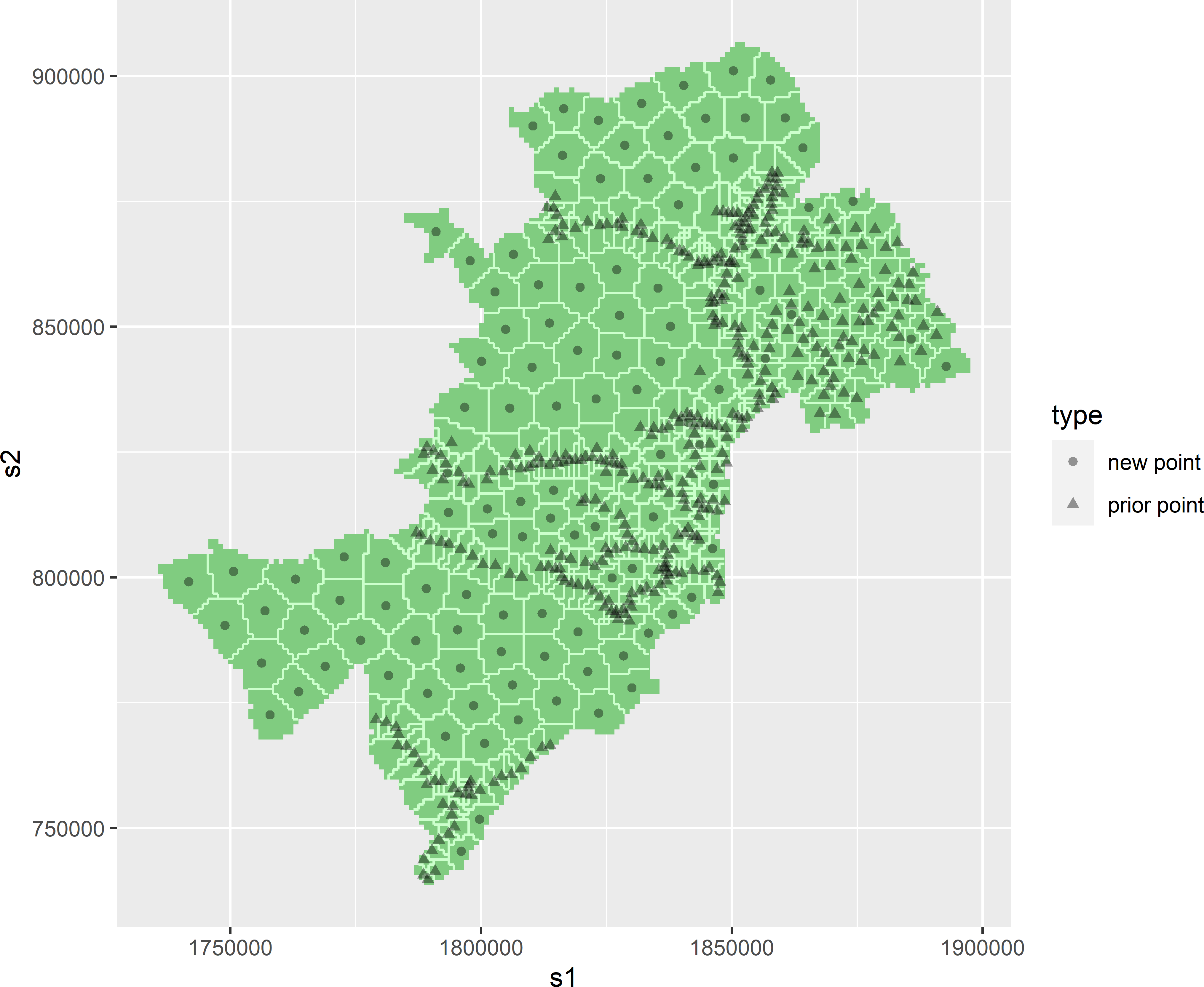

Figure 17.5: Spatial infill sample of 100 points from West-Amhara.

In the output object of spsample, both the prior and the new sampling points are included. The new points can be obtained as follows:

units <- which(mysample@isPriorPoint == FALSE)
mysample <- as(mysample, "data.frame")
mysample_new <- mysample[units, ]

Exercises

6. Write an R script to select a spatial infill sample of size 100 from study area Xuancheng in China. Use the iPSM sample in tibble sampleXuancheng of package sswr as a legacy sample. To map the SOM concentration, we want to measure the SOM concentration at 100 more sampling points.
   • Read the file data/Elevation_Xuancheng.rds with function rast of package terra, and use this file as a discretisation of the study area.
   • For computational reasons, there are far too many raster cells. That many cells are not needed to select a spatial infill sample. Subsample the raster file by selecting a square grid with a spacing of 900 m \(\times\) 900 m. First, convert the SpatRaster object to a data.frame, and then change it to a SpatialPixelsDataFrame using function gridded. Then use function spsample with argument type = "regular".
   • Select a spatial infill sample using functions stratify and sample of package spcosa.

References

Brus, D. J., J. J. de Gruijter, and J. W. van Groenigen. 2007. “Designing Spatial Coverage Samples Using the k-means Clustering Algorithm.” In Digital Soil Mapping. An Introductory Perspective, edited by P. Lagacherie, A. B. McBratney, and M. Voltz, 183–92. Elsevier.

Pebesma, E. J., and R. S. Bivand. 2005. “Classes and methods for spatial data in R.” R News 5 (2): 9–13. http://cran.r-project.org/doc/Rnews/.

Walvoort, D. J. J., D. J. Brus, and J. J. de Gruijter. 2010. “An R Package for Spatial Coverage Sampling and Random Sampling from Compact Geographical Strata by k-Means.” Computers & Geosciences 36 (10): 1261–67. https://doi.org/10.1016/j.cageo.2010.04.005.