Chapter 18 Covariate space coverage sampling

Regular grid sampling and spatial coverage sampling are pure spatial sampling designs. Covariates possibly related to the study variable are not accounted for in selecting sampling units. This can be suboptimal when the study variable is related to covariates of which maps are available, think for instance of remote sensing imagery or digital elevation models related to soil properties. Maps of these covariates can be used in mapping the study variable by, for instance, a multiple linear regression model or a random forest. This chapter describes a simple, straightforward method for selecting sampling units on the basis of the covariate values of the raster cells.

The simplest option for covariate space coverage (CSC) sampling is to cluster the raster cells by the k-means clustering algorithm in covariate space. Similar to spatial coverage sampling (Section 17.2) the mean squared shortest distance (MSSD) is minimised, but now the distance is not measured in geographical space but in a \(p\)-dimensional space spanned by the \(p\) covariates. Think of this space as a multidimensional scatter plot with the covariates along the axes. The covariates are centred and scaled so that their means become zero and standard deviations become one. This is needed because, contrary to the spatial coordinates used as clustering variables in spatial coverage sampling, the ranges of the covariates in the population can differ greatly. In the clustering of the raster cells, the mean squared shortest scaled distance (MSSSD) is minimised. The name ‘scaled distance’ can be confusing. The distances are not scaled, but rather they are computed in a space spanned by the scaled covariates.

In the next code chunk, a CSC sample of 20 units is selected from Eastern Amazonia. All five quantitative covariates, SWIR2, Terra_PP, Prec_dm, Elevation, and Clay, are used as covariates. To select 20 units, 20 clusters are constructed using function kmeans of the stats package (R Core Team 2021). The number of clusters is passed to function kmeans with argument centers. Note that the number of clusters is not based, as would be usual in cluster analysis, on the assumed number of subregions with a high density of units in the multivariate distribution, but rather on the number of sampling units. The k-means clustering algorithm is a deterministic algorithm, i.e., the final optimised clustering is fully determined by the initial clustering. This final clustering can be suboptimal, i.e., the minimised MSSSD value is somewhat larger than the global minimum. Therefore, the clustering should be repeated many times, every time starting with a different random initial clustering. The number of repeats is specified with argument nstart. The best solution is automatically kept. To speed up the computations, a 5 km \(\times\) 5 km subgrid of grdAmazonia is used.

covs <-  c("SWIR2", "Terra_PP", "Prec_dm", "Elevation", "Clay")
n <- 20
set.seed(314)
myclusters <- kmeans(
  scale(grdAmazonia[, covs]), centers = n, iter.max = 10000, nstart = 100)
grdAmazonia$cluster <- myclusters$cluster

Raster cells with the shortest scaled Euclidean distance in covariate space to the centres of the clusters are selected as the sampling units. To this end, first a matrix with the distances of all the raster cells to the cluster centres is computed with function rdist of package fields (Nychka et al. 2021). The raster cells closest to the centres are computed with function apply, using argument FUN = which.min.

library(fields)
covs_s <- scale(grdAmazonia[, covs])
D <- rdist(x1 = myclusters$centers, x2 = covs_s)
units <- apply(D, MARGIN = 1, FUN = which.min)
myCSCsample <- grdAmazonia[units, ]

Figure 18.1 shows the clustering of the raster cells and the raster cells closest in covariate space to the centres that are used as the selected sample. In Figure 18.2 the selected sample is plotted in biplots of some pairs of covariates. In the biplots, some sampling units are clearly clustered. However, this is misleading, as actually we must look in five-dimensional space to see whether the units are clustered. Two units with a large separation distance in a five-dimensional space can look quite close when projected on a two-dimensional plane.

The next code chunk shows how the MSSSD of the selected sample can be computed.

D <- rdist(x1 = scale(
  myCSCsample[, covs], center = attr(covs_s, "scaled:center"),
  scale = attr(covs_s, "scaled:scale")), x2 = covs_s)
dmin <- apply(D, MARGIN = 2, min)
MSSSD <- mean(dmin^2)

Note that to centre and scale the covariate values in the CSC sample, the population means and the population standard deviations are used, as passed to function scale with arguments center and scale. If these means and standard deviations are unspecified, the sample means and the sample standard deviations are used, resulting in an incorrect value of the minimised MSSSD value. The MSSSD of the selected sample equals 1.004.

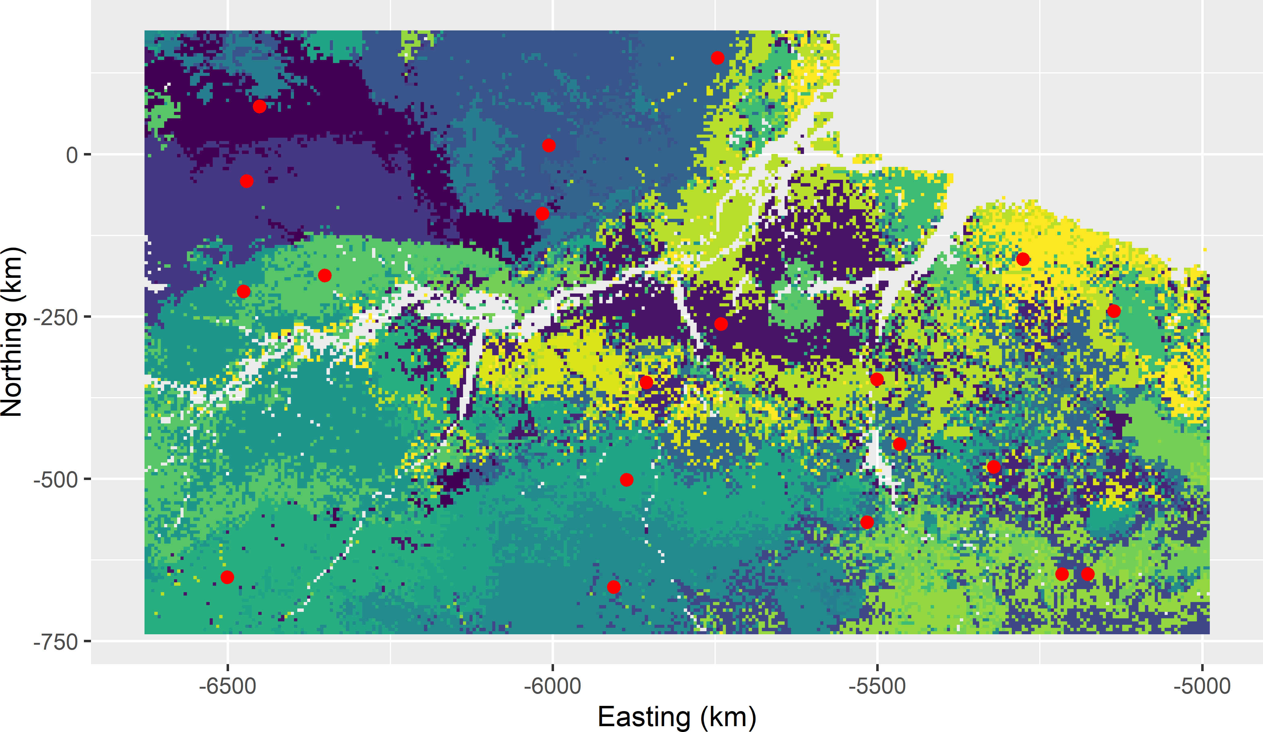
Figure 18.1: Covariate space coverage sample of 20 units from Eastern Amazonia, obtained with k-means clustering using five covariates, plotted on a map of the clusters.

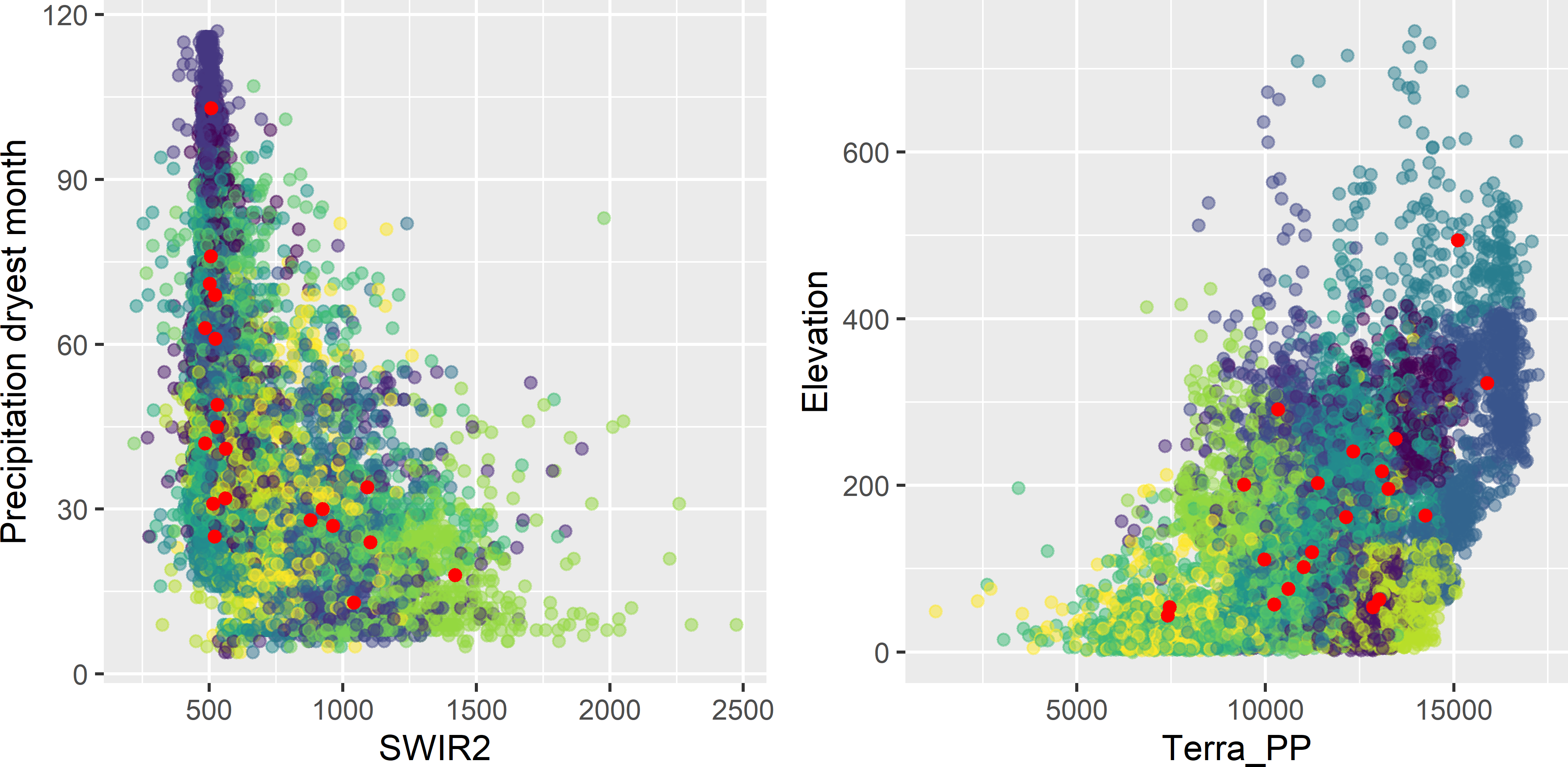
Figure 18.2: Covariate space coverage sample of Figure 18.1 plotted in biplots of covariates, coloured by cluster.

Instead of function kmeans we may use function kmeanspp of package LICORS (Goerg 2013). This function is an implementation of the k-means++ algorithm (Arthur and Vassilvitskii 2007). This algorithm consists of two parts, namely the selection of an optimised initial sample, followed by the standard k-means. The algorithm is as follows:

1. Select one unit (raster cell) at random.
   
2. For each unsampled unit \(j\), compute \(d_{kj}\), i.e., the distance in standardised covariate space between \(j\) and the nearest unit \(k\) that has already been selected.
   
3. Choose one new raster cell at random as a new sampling unit with probabilities proportional to \(d^2_{kj}\) and add the selected raster cell to the set of selected cells.
   
4. Repeat steps 2 and 3 until \(n\) centres have been selected.
   
5. Now that the initial centres have been selected, proceed using standard k-means.

library(LICORS)
myclusters <- kmeanspp(
  scale(grdAmazonia[, covs]), k = n, iter.max = 10000, nstart = 30)

Due to the improved initial centres, the risk of ending in a local minimum is reduced. The k-means++ algorithm is of interest for small sample sizes. For large sample sizes, the extra time needed for computing the initial centres can become substantial and may not outweigh the larger number of starts that can be afforded with the usual k-means algorithm for the same computing time.

18.1 Covariate space infill sampling

If we have legacy data that can be used to fit a model for mapping, it is more efficient to select an infill sample, similar to spatial infill sampling explained in Section 17.3. The only difference with spatial infill sampling is that the legacy data are now plotted in the space spanned by the covariates. The empty regions we would like to fill in are now the undersampled regions in this covariate space. The legacy sample units serve as fixed cluster centres; they cannot move through the covariate space during the optimisation of the infill sample. In the next code chunk, a function is defined for covariate space infill sampling.

CSIS <- function(fixed, nsup, nstarts, mygrd) {
  n_fix <- nrow(fixed)
  p <- ncol(mygrd)
  units <- fixed$units
  mygrd_minfx <- mygrd[-units, ]
  MSSSD_cur <- NA
  for (s in 1:nstarts) {
    units <- sample(nrow(mygrd_minfx), nsup)
    centers_sup <- mygrd_minfx[units, ]
    centers <- rbind(fixed[, names(mygrd)], centers_sup)
    repeat {
      D <- rdist(x1 = centers, x2 = mygrd)
      clusters <- apply(X = D, MARGIN = 2, FUN = which.min) %>% as.factor(.)
      centers_cur <- centers
      for (i in 1:p) {
        centers[, i] <- tapply(mygrd[, i], INDEX = clusters, FUN = mean)
      }
      #restore fixed centers
      centers[1:n_fix, ] <- centers_cur[1:n_fix, ]
      #check convergence
      sumd <- diag(rdist(x1 = centers, x2 = centers_cur)) %>% sum(.)
      if (sumd < 1E-12) {
        D <- rdist(x1 = centers, x2 = mygrd)
        Dmin <- apply(X = D, MARGIN = 2, FUN = min)
        MSSSD <- mean(Dmin^2)
        if (s == 1 | MSSSD < MSSSD_cur) {
          centers_best <- centers
          clusters_best <- clusters
          MSSSD_cur <- MSSSD
        }
        break
      }
    }
  }
  list(centers = centers_best, clusters = clusters_best)
}

The function is used to select an infill sample of 15 units from Eastern Amazonia. A legacy sample of five units is randomly selected.

set.seed(314)
units <- sample(nrow(grdAmazonia), 5)
fixed <- data.frame(units, scale(grdAmazonia[, covs])[units, ])
mygrd <- data.frame(scale(grdAmazonia[, covs]))
res <- CSIS(fixed = fixed, nsup = 15, nstarts = 10, mygrd = mygrd)

Figures 18.3 and 18.4 show the selected sample plotted on a map of the clusters and in biplots of covariates, respectively.

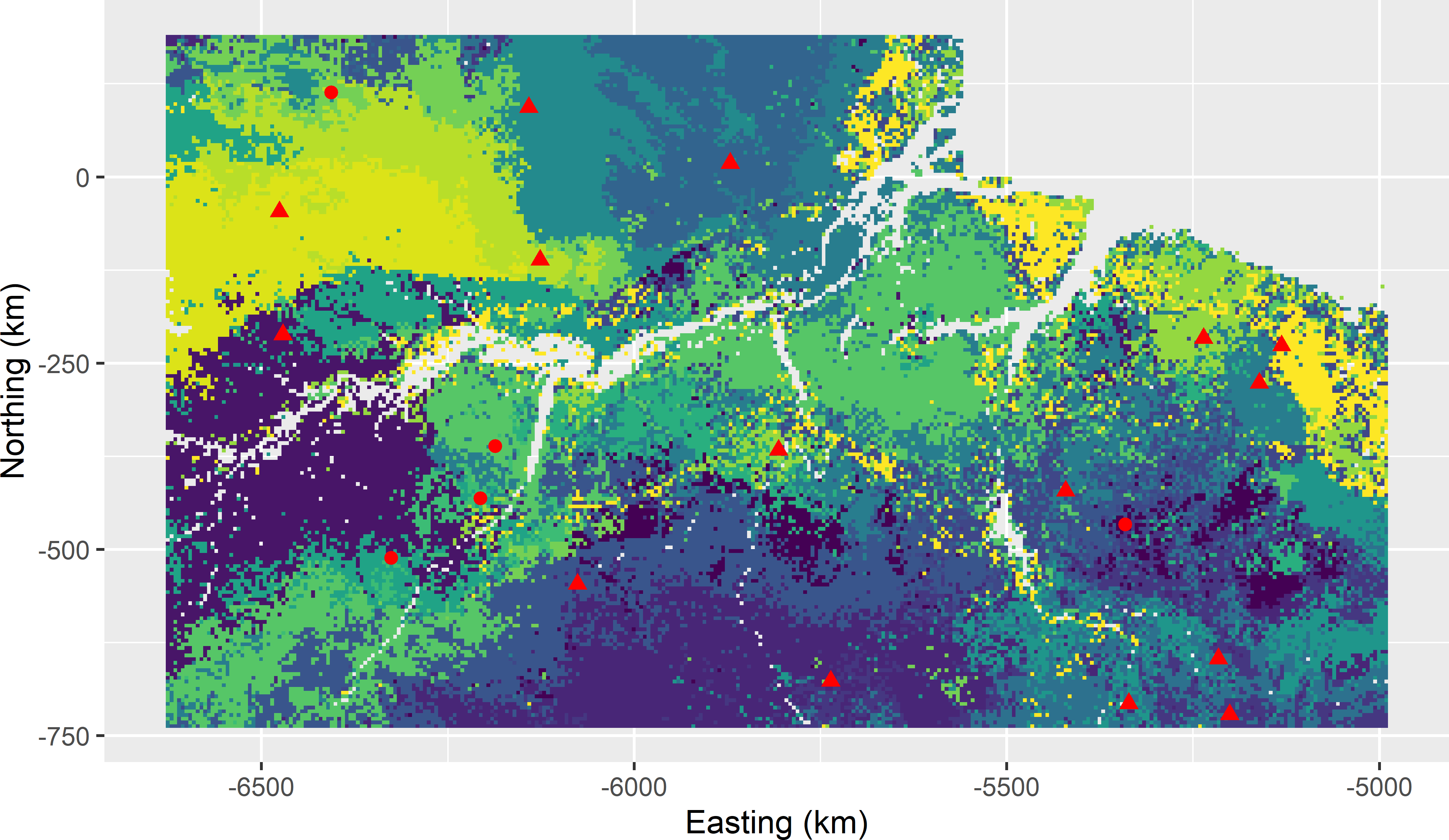
Figure 18.3: Covariate space infill sample of 15 units from Eastern Amazonia, obtained with k-means clustering and five fixed cluster centres, plotted on a map of the clusters. The dots represent the fixed centres (legacy sample), the triangles the infill sample.

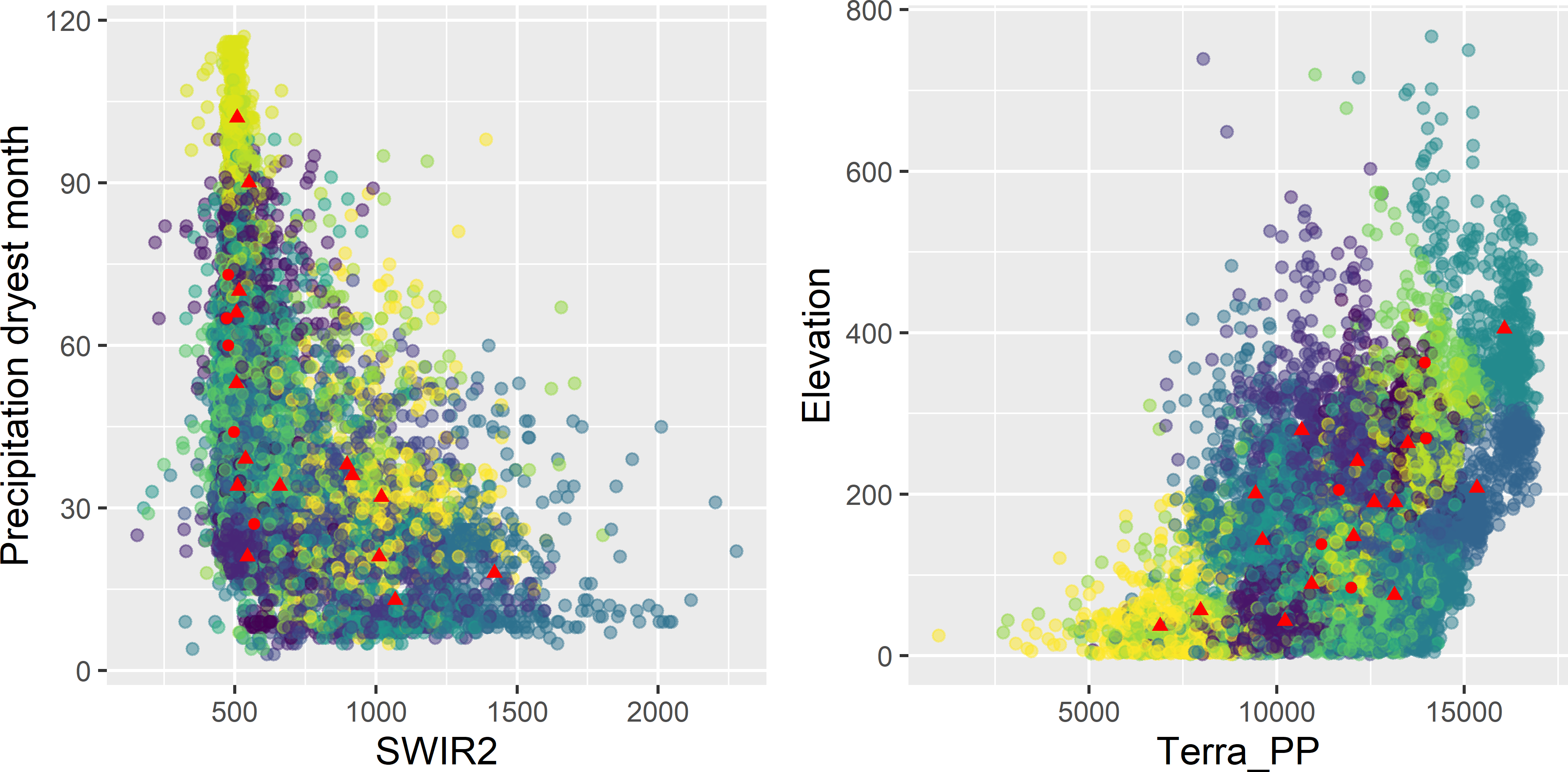
Figure 18.4: Covariate space infill sample of Figure 18.3 plotted in biplots of covariates, coloured by cluster. The dots represent the fixed centres (legacy sample), the triangles the infill sample.

18.2 Performance of covariate space coverage sampling in random forest prediction

CSC sampling can be a good candidate for a sampling design if we have multiple maps of covariates, and in addition if we do not want to rely on a linear relation between the study variable and the covariates. In this situation, we may consider mapping with machine learning algorithms such as neural networks and random forests (RF).

I used the Eastern Amazonia data set to evaluate CSC sampling for mapping the aboveground biomass (AGB). The five covariates are used as predictors in RF modelling. The calibrated models are used to predict AGB at the units of a validation sample of size 25,000 selected by simple random sampling without replacement from the 1 km \(\times\) 1 km grid, excluding the cells of the 10 km \(\times\) 10 km grid from which the calibration samples are selected. The predicted AGB values at the validation units are compared with the true AGB values, and the prediction errors are computed. The sample mean of the squared prediction error is a design-unbiased estimator of the population mean squared error, i.e., the mean of the squared errors at all population units (excluding the units of the 10 km \(\times\) 10 km grid), see Chapter 25.

Three sample sizes are used, \(n=\) 25, 50, 100. Of each sample size, 500 CSC samples are selected using the k-means algorithm, leading to 1,500 CSC samples in total. The numbers of starts are 500, 350, and 200 for \(n=\) 25, 50, and 100, respectively. With these numbers of starts, the computing time was about equal to conditioned Latin hypercube sampling, see next chapter. Each sample is used to calibrate a RF model. Simple random sampling (SI) is used as a reference sampling design that ignores the covariates.

In Figure 18.5 the root mean squared error (RMSE) of the RF predictions of AGB is plotted against the minimised MSSSD, both for the \(3 \times 500\) CSC samples and for the 3 \(\times\) 500 simple random samples. It is no surprise that for all three sample sizes the minimised MSSSD values of the CSC samples are substantially smaller than those of the SI samples. However, despite the substantial smaller MSSSD values, the RMSE values for the CSC samples are only a bit smaller than those of the SI samples. Only for \(n=50\) a moderately strong positive correlation can be seen: \(r=0.513\). For \(n=25\) the correlation is 0.264 only, and for \(n=100\) it is even negative: \(r=-0.183\). On average in this case study, CSC and SI perform about equally (Table 18.1). However, especially with \(n=25\) and 50 the sampling distribution of RMSE with SI has a long right tail. This implies that with SI there is a serious risk that a sample will be selected resulting in poor RF predictions of AGB. In Chapter 19 CSC sampling is compared with conditioned Latin hypercube sampling.

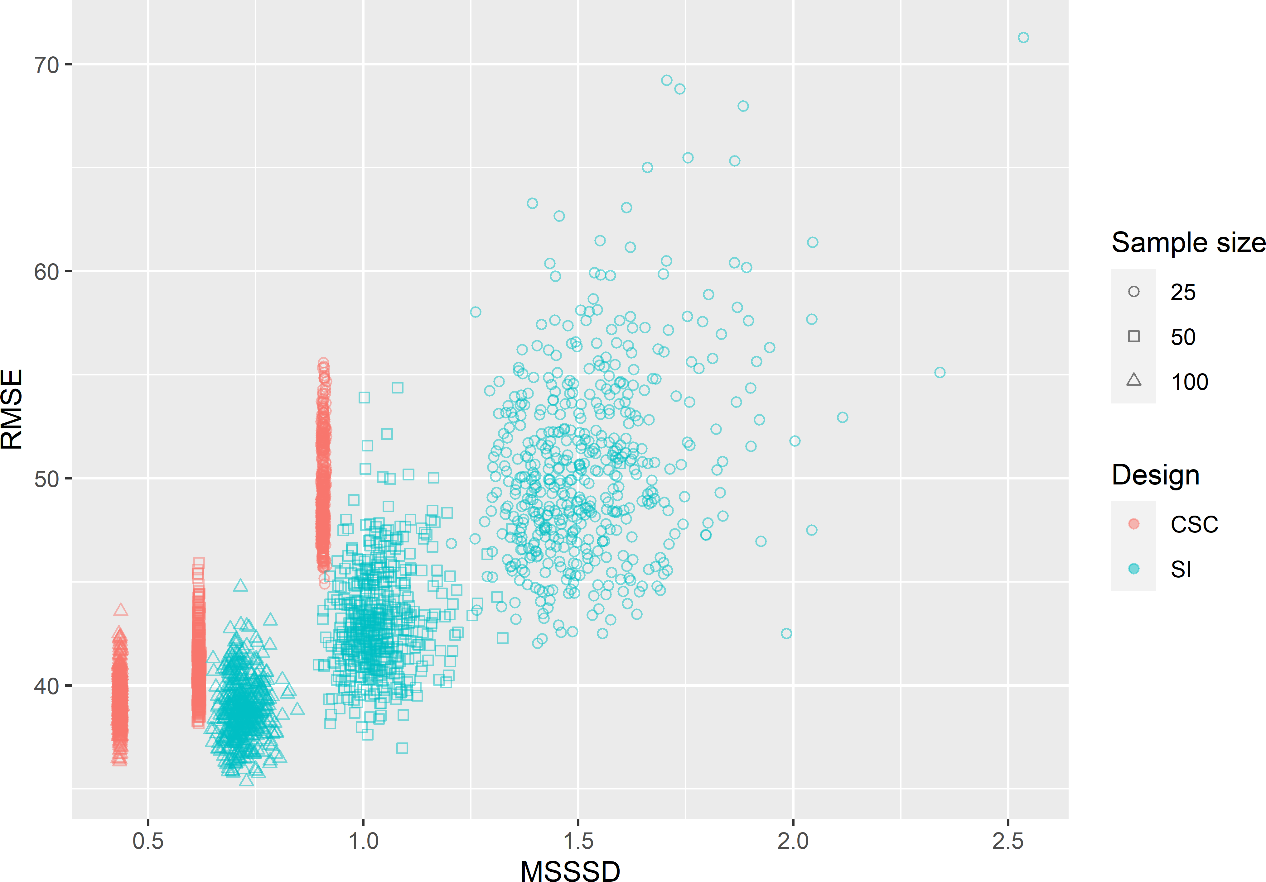
Figure 18.5: Scatter plot of the minimisation criterion MSSSD and the root mean squared error (RMSE) of RF predictions of AGB in Eastern Amazonia for covariate space coverage (CSC) sampling and simple random (SI) sampling, and three sample sizes.

Table 18.1: Mean RMSE of RF predictions of AGB in Eastern Amazonia of 500 covariate space coverage (CSC) samples and 500 simple random (SI) samples, for three sample sizes.

Sample size	CSC	SI
25	49.30	50.58
50	40.85	43.16
100	39.33	38.83

Exercises

1. Write an R script to select a covariate space coverage sample of size 20 from Hunter Valley (grdHunterValley of package sswr). Use the covariates cti (compound topographic index, which is the same as topographic wetness index), ndvi (normalised difference vegetation index), and elevation_m in k-means clustering of the raster cells. Plot the clusters and the sample on a map of cti and in a biplot of cti against ndvi.

References

Arthur, D., and S. Vassilvitskii. 2007. “k-means++: The advantages of careful seeding.” Proceedings of the Annual ACM-SIAM Symposium on Discrete Algorithms 07-09-January-2007: 1027–35.

Goerg, G. M. 2013. LICORS: Light Cone Reconstruction of States - Predictive State Estimation From Spatio-Temporal Data. https://CRAN.R-project.org/package=LICORS.

Nychka, D., R. Furrer, J. Paige, S. Sain, F. Gerber, and M. Iverson. 2021. Fields: Tools for Spatial Data. Boulder, CO, USA: University Corporation for Atmospheric Research. https://github.com/dnychka/fieldsRPackage.

R Core Team. 2021. R: A Language and Environment for Statistical Computing. Vienna, Austria: R Foundation for Statistical Computing. https://www.R-project.org/.