Chapter 16 Introduction to sampling for mapping
16.1 When is probability sampling not required?
This second part of the book deals with sampling for mapping, i.e., for predicting the study variable at the nodes of a fine discretisation grid. For mapping, a model-based sampling approach is the most natural option. When a statistical model, i.e., a model containing an error term modelled by a probability distribution, is used to map the study variable from the sample data, selection of the sampling units by probability sampling is not strictly needed anymore in order to make statistical statements about the population, i.e., statements with quantified uncertainty, see Section 1.2. As a consequence, there is room for optimising the sampling units by searching for those units that lead to the most accurate map, for instance, the map with the smallest squared prediction error averaged over all locations in the mapped study area, see Chapter 25.
As an illustration, consider the following statistical model to be used for mapping: a simple linear regression model for the study variable to be mapped:
\[\begin{equation} Z_k = \beta_0 + \beta_1 x_k + \epsilon_k \;, \tag{16.1} \end{equation}\]
with \(Z_k\) the study variable of unit \(k\), \(\beta_0\) and \(\beta_1\) regression coefficients, \(x_k\) a covariate for unit \(k\) used as a predictor, and \(\epsilon_k\) the error (residual) at unit \(k\), normally distributed with mean zero and a constant variance \(\sigma^2\). The errors are assumed independent, so that \(\text{Cov}(\epsilon_k,\epsilon_j)=0\) for all \(k \neq j\). Figure 16.1 shows a simple random sample without replacement and the sample optimised for mapping with a simple linear regression model. Both samples are plotted on a map of the covariate \(x\).
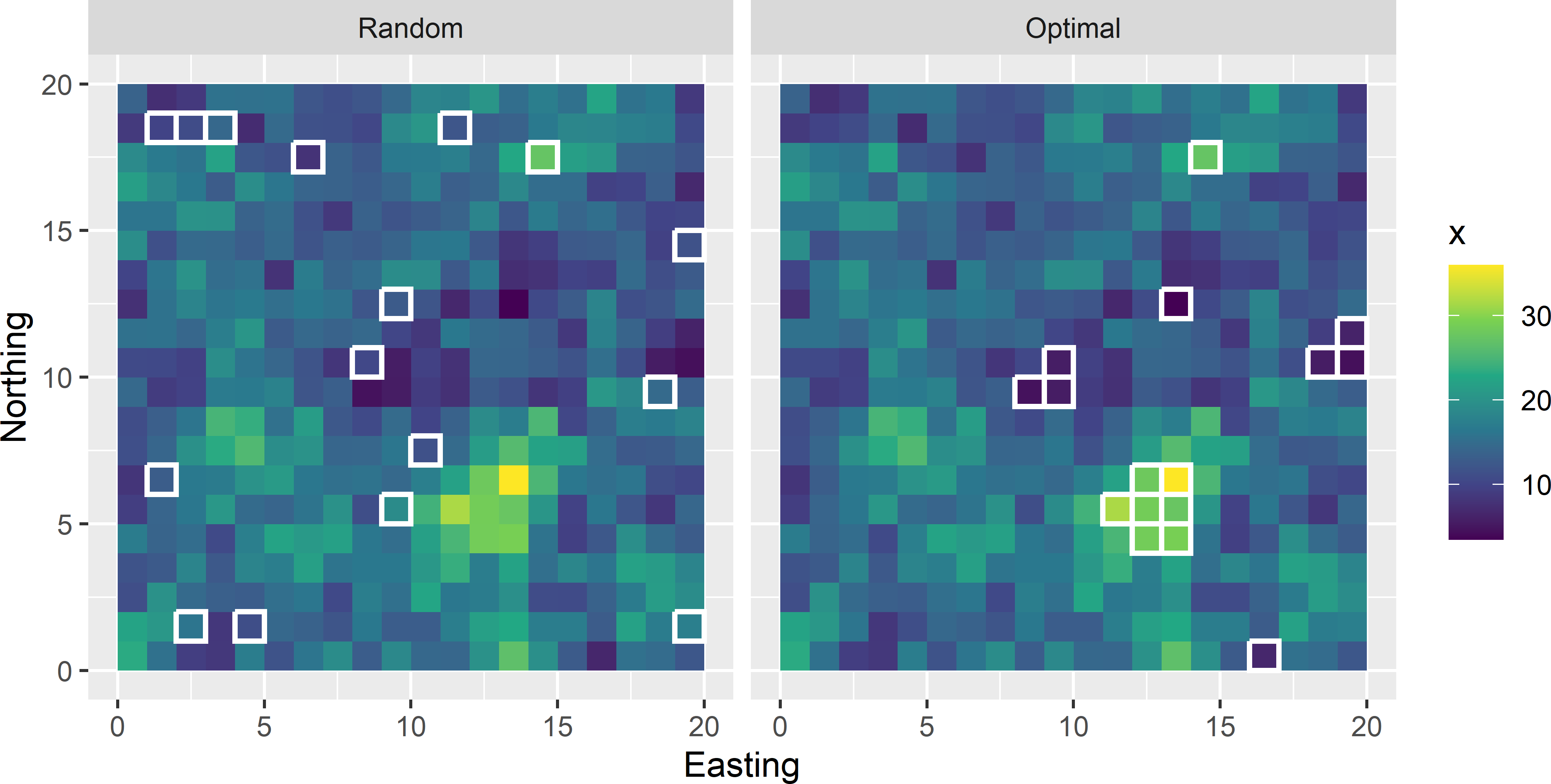
Figure 16.1: Simple random sample and optimal sample for mapping with a simple linear regression model, plotted on a map of the covariate.
The optimal sample for mapping with a simple linear regression model contains the units with the smallest and the largest values of the covariate \(x\). The optimal sample shows strong spatial clustering. Spatial clustering is not avoided because in a simple linear regression model we assume that the residuals are not spatially correlated. In Chapter 23 I will show that when the residuals are spatially correlated, spatial clustering of sampling units is avoided. The standard errors of both regression coefficients are considerably smaller for the optimal sample (Table 16.1). The joint uncertainty about the two regression coefficients, quantified by the determinant of the variance-covariance matrix of the regression coefficient estimators, is also much smaller for the optimal sample. When we are less uncertain about the regression coefficients, we are also less uncertain about the regression model predictions of the study variable \(z\) at points where we have observations of the covariate \(x\) only. We can conclude that for mapping with a simple linear regression model, in this example simple random sampling is not a good option.
| Sampling design | se intercept | se slope | Determinant |
|---|---|---|---|
| SI | 1.70 | 0.118 | 0.003876 |
| Optimal | 1.06 | 0.050 | 0.000940 |
Of course, this simple example would only be applicable if we have evidence of a linear relation between study variable \(z\) and covariate \(x\), and in addition if we are willing to rely on the assumption that the residuals are not spatially correlated.
16.2 Sampling for simultaneously mapping and estimating means
Although probability sampling is not strictly needed for mapping with a statistical model, in some situations, when feasible, it can still be advantageous to select a probability sample. If the aim of the survey is to map the study variable, as well as to estimate the mean or total for the entire study area or for several subareas, probability sampling can be a good option. Think, for instance, of sampling for the dual objectives of mapping and at the same time estimating soil carbon stocks. Although the statistical model used for mapping can also be used for model-based prediction of the total carbon stocks in the study area and subareas (Section 14.3), we may prefer to estimate these totals by design-based or model-assisted inference. The advantage of design-based and model-assisted estimation of these totals is their validity. Validity means that an objective assessment of the uncertainty of the estimated mean or total is warranted, and that the coverage of confidence intervals is (almost) correct, provided that the sample is large enough to assume an approximately normal distribution of the estimator and design-unbiasedness of the variance estimator, see Chapter 26. In design-based estimation, no model of the spatial variation is used. Therefore, discussions are avoided about how realistic modelling assumptions are. In model-assisted estimation, these discussions are irrelevant as well, because we do not rely on these assumptions. A poor model results in large variances of the estimated mean or total and, as a consequence, a wide confidence interval, so that the coverage of the confidence interval is in agreement with the nominal coverage, see Section 26.6 for more details.
The question then is: what is a suitable probability sampling design for both aims? First, I would recommend a sampling design with equal inclusion probabilities. This is because in standard model-based inference unequal inclusion probabilities are not accounted for, which may lead to systematic prediction errors when small or large values are overrepresented in the sample (Section 26.3).
Second, in case we have subareas of which we would like to estimate the mean or total (domains of interest), using these subareas as strata in stratified random sampling makes sense, unless there are too many. This requires that of all population units (nodes of discretisation grid) we must know to which subarea it belongs, so that this information can be added to the sampling frame.
Third, a sampling design spreading the sampling units in geographical space is attractive as well, for instance through compact geographical stratification (Section 4.6) or sampling with the local pivotal method (Subsection 9.2.1). We may profit from this geographical spreading if some version of kriging is used for mapping (Chapter 21). In addition, the geographical spreading may enhance the coverage of the space spanned by covariates related to the study variable. Spreading in covariate space can also be explicitly accounted for using the covariates as spreading variables in the local pivotal method.
As an illustration, I selected a single sample of 500 units from Eastern Amazonia with the dual aim of mapping aboveground biomass (AGB) as well as estimating the means of AGB for four biomes. The biomes are used as strata in stratified random sampling. First, the stratum sample sizes are computed for proportional allocation, so that the inclusion probabilities are approximately equal for all population units.
grdAmazonia$Biome <- as.factor(grdAmazonia$Biome)
biomes <- c("Mangrove", "Forest_dry", "Grassland", "Forest_moist")
levels(grdAmazonia$Biome) <- biomes
N_h <-  table(grdAmazonia$Biome)
n <- 500
n_h <- round(n * N_h / sum(N_h))
n_h[3] <- n_h[3] + 1
print(n_h)
    Mangrove   Forest_dry    Grassland Forest_moist
           2           11           28          459
Biome Forest_moist is by far the largest biome with a sample size of 459 points.
In the next code chunk, a balanced sample is selected with equal inclusion probabilities, using both the categorical variable biome and the continuous variable lnSWIR2 as balancing variables (Subsection 9.1.3). The geographical coordinates are used as spreading variables.
library(BalancedSampling)
grdAmazonia$lnSWIR2 <- log(grdAmazonia$SWIR2)
pi <- n_h / N_h
stratalabels <- levels(grdAmazonia$Biome)
lut <- data.frame(Biome = stratalabels, pi = as.numeric(pi))
grdAmazonia <- merge(x = grdAmazonia, y = lut)
Xbal <- model.matrix(~ Biome - 1, data = grdAmazonia) %>%
  cbind(grdAmazonia$lnSWIR2)
Xspread <- cbind(grdAmazonia$x1, grdAmazonia$x2)
set.seed(314)
units <- lcube(Xbal = Xbal, Xspread = Xspread, prob = grdAmazonia$pi)
mysample <- grdAmazonia[units, ]
Figure 16.2 shows the selected sample.
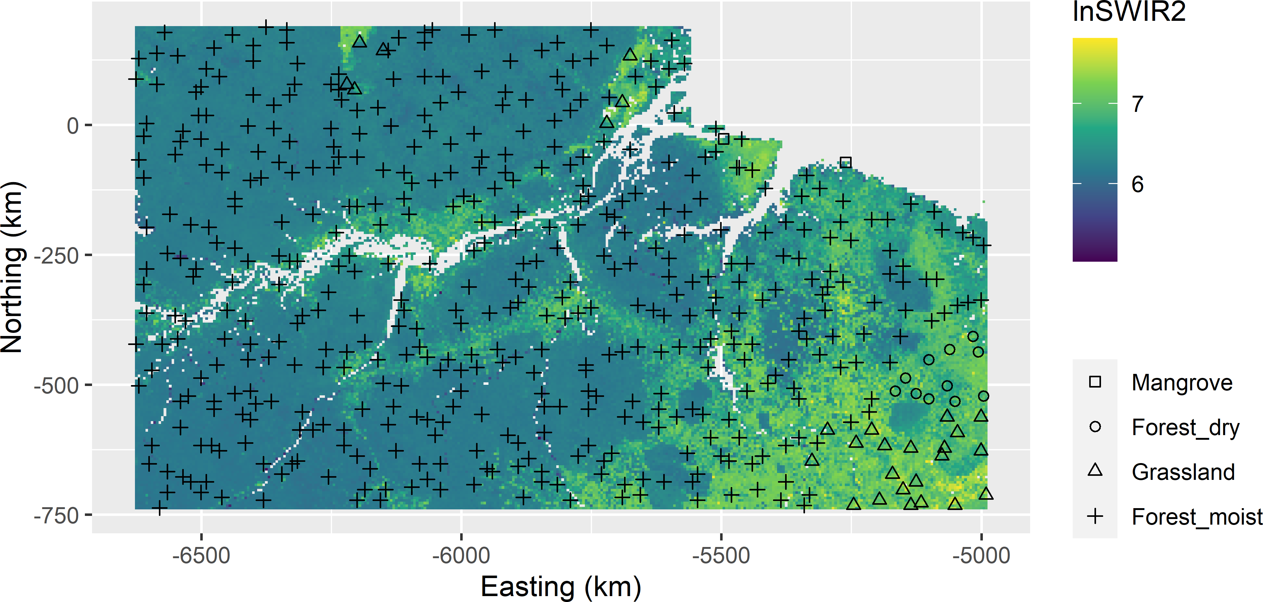
Figure 16.2: Balanced sample of size 500 from Eastern Amazonia, balanced on biome and lnSWIR2, with geographical spreading. Equal inclusion probabilities are used.
I think this is a suitable sample, both for mapping AGB across the entire study area, for instance by kriging with an external drift (Section 21.3), and for estimating the mean AGB of the four biomes. For biome Forest_moist, the population mean can be estimated from the data of this biome only, using the \(\pi\) estimator, as the sample size of this biome is very large (Section 9.3). For the other three biomes, we may prefer model-assisted estimation for small domains as described in Section 14.2.
In this example I used one quantitative covariate, lnSWIR2, for balancing the sample. If we have a legacy sample that can be used to fit a linear or non-linear model, for instance a random forest using multiple covariates and factors as predictors (Chapter 10), then this model can be used to predict the study variable for all population units, so that we can use the predictions of the study variable to balance the sample, see Section 10.4.
16.3 Broad overview of sampling designs for mapping
The non-probability sampling designs for mapping described in the following chapters can be grouped into three categories (Brus 2019):
- geometric sampling designs (Chapters 17 and 18);
- adapted experimental designs (Chapters 19 and 20); and
- model-based sampling designs (Chapters 22 and 23).
Square and triangular grids are examples of geometric sampling designs; the sampling units show a regular, geometric spatial pattern. In other geometric sampling designs the spatial pattern is not perfectly regular. Yet these are classified as geometric sampling designs when the samples are obtained by minimising some geometric criterion, i.e., a criterion defined in terms of distances between the sampling units and the nodes of a fine prediction grid discretising the study area (Section 17.2 and Chapter 18).
In model-based sampling designs, the samples are obtained by minimising a criterion that is defined in terms of variances of prediction errors. An example is the mean kriging variance criterion, i.e., the average of the kriging variances over all nodes of the prediction grid. Model-based sampling therefore requires prior knowledge of the model of spatial variation. Such a model must be specified and justified. Once this model is given, the sample can be optimised. In Chapter 22 I will show how a spatial model can be used to optimise the spacing of a square grid given a requirement on the accuracy of the map. The grid spacing determines the number of sampling units, so this optimisation boils down to determining the required sample size. In Chapter 23 I will show how a sample of a given size can be further optimised through optimisation of the spatial coordinates of the sampling units.
In Chapter 1 the design-based and model-based approaches for sampling and statistical inference were introduced. Note that a model-based approach does not necessarily imply model-based sampling. The adjective ‘model-based’ refers to the model-based inference, not to the selection of the units. In a model-based approach sampling units can be, but need not be, selected by model-based sampling. If they are, then both in selecting the units and in mapping a statistical model is used. In most cases, the two models differ: once the sample data are collected, these are used to update the postulated model used for designing the sample. The updated model is then used in mapping.
Besides geometric and model-based sampling designs for a spatial survey, a third category can be distinguished: sampling designs that are adaptations of experimental designs. An adaptation is necessary because in contrast to experiments, in observational studies one is not free to choose combinations of levels of different factors. For instance, when two covariates are strongly positively correlated, it may happen that there are no units with a relatively large value for one covariate and a relatively small value for the other covariate.
In a full factorial design, all combinations of factor levels are observed. For instance, suppose we have only two covariates, e.g., application rates for N and P in an agricultural experiment, and four levels for each covariate. To account for possible non-linear effects, a good option is to have multiple plots for all 4 \(\times\) 4 combinations. This is referred to as a full factorial design. With \(k\) factors and \(l\) levels per factor the total number of observations is \(l^k\). With numerous factors and/or numerous levels per factor, this becomes unfeasible in practice. Alternative designs have been developed that need fewer observations but still provide detailed information about how the study variable responds to changes in the factor levels. Examples are Latin hypercube samples and response surface designs. The survey sampling analogues of these experimental designs are described in Chapters 19 and 20.