Chapter 22 Model-based optimisation of the grid spacing

This is the first chapter on model-based sampling¹². In Section 17.2 and Chapter 18 a geometric criterion is minimised, i.e., a criterion defined in terms of distances, either in geographic space (Section 17.2) or in covariate space (Chapter 18). In model-based sampling, the minimisation criterion is a function of the variance of the prediction errors.

This chapter on model-based sampling is about optimisation of the spacing of a square grid, i.e., the distance between neighbouring points in the grid. The grid spacing is derived from a requirement on the accuracy of the map. Here and in following chapters, I assume that the map is constructed by kriging; see Chapter 21 for an introduction. As we have seen in Chapter 21, a kriging prediction of the study variable at an unobserved location is accompanied by a variance of the prediction error, referred to as the kriging variance. The map accuracy requirement is a population parameter of this kriging variance, e.g., the population mean of the kriging variance.

22.1 Optimal grid spacing for ordinary kriging

Suppose that we require the population mean of the kriging variance not to exceed a given threshold. The question then is what the tolerable or maximum possible grid spacing is, given this requirement. For finding the tolerable grid spacing we must have prior knowledge of the spatial variation. I first consider the situation in which it is reasonable to assume that the model-mean of the study variable is constant throughout the study area, but is unknown. When the model-mean is unknown, ordinary kriging (OK) is used for mapping. Furthermore, we need a semivariogram of the study variable. In practice, we often do not have a reliable estimate of the semivariogram. In the best case scenario, we have some existing data, of sufficient quantity and suitable spatial distribution, that can be used to estimate the semivariogram. In other cases, such data are lacking and a best guess of the semivariogram must be made, for instance using data for the same study variable from other, similar areas.

There is no simple equation that relates the grid spacing to the kriging variance. What can be done is calculate the mean OK variance for a range of grid spacings, plot the mean ordinary kriging variances against the grid spacings, and use this plot inversely to determine the tolerable grid spacing, given a constraint on the mean OK variance.

In the next code chunks, this procedure is used to compute the tolerable spacing of a square grid for mapping soil organic matter (SOM) in West-Amhara. The legacy data of the SOM concentration (dag kg^-1), used before to design a spatial infill sample (Section 17.3), are used here to estimate a semivariogram. A sample semivariogram is estimated by the method-of-moments (MoM), and a spherical model is fitted using functions of package gstat (E. J. Pebesma 2004). The values for the partial sill, range, and nugget, passed to function fit.variogram with argument model, are guesses from an eyeball examination of the sample semivariogram obtained with function variogram, see Figure 22.1. The ultimate estimates of the semivariogram parameters differ from these eyeball estimates. First, the projected coordinates of the sampling points are changed from m into km using function mutate¹³.

library(gstat)
grdAmhara <- grdAmhara %>%
  mutate(s1 = s1 / 1000, s2 = s2 / 1000)
sampleAmhara <- sampleAmhara %>%
  mutate(s1 = s1 / 1000, s2 = s2 / 1000)
coordinates(sampleAmhara) <- ~ s1 + s2
vg <- variogram(SOM ~ 1, data = sampleAmhara)
model_eye <- vgm(model = "Sph", psill = 0.6, range = 40, nugget = 0.6)
vgm_MoM <- fit.variogram(vg, model = model_eye)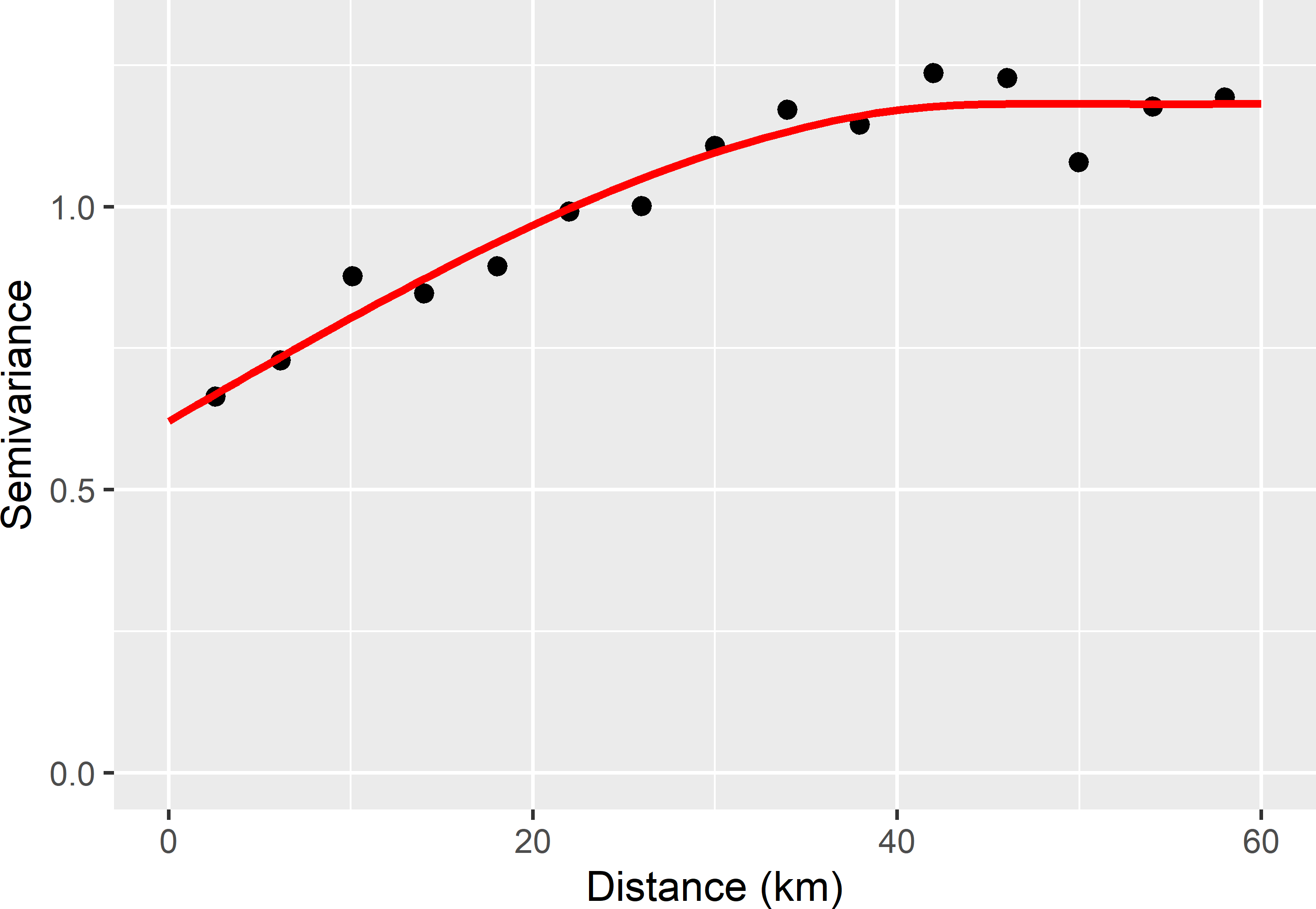

Figure 22.1: Sample semivariogram and fitted spherical model of the SOM concentration in West-Amhara, estimated from the legacy data.

The semivariogram of SOM can also be estimated by maximum likelihood (ML) using function likfit of package geoR (Ribeiro Jr et al. 2020), see Section 21.4.

library(geoR)
sampleAmhara <- as_tibble(sampleAmhara)
dGeoR <- as.geodata(
  obj = sampleAmhara, header = TRUE, coords.col = c("s1", "s2"),
  data.col = "SOM")
vgm_ML <- likfit(geodata = dGeoR, trend = "cte",
  cov.model = "spherical", ini.cov.pars = c(0.6, 40),
  nugget = 0.6, lik.method = "ML", messages = FALSE)

Table 22.1 shows the ML estimates of the parameters of the spherical semivariogram, together with the MoM estimates. Either could be used in the following steps.

Table 22.1: Method-of-moments (MoM) and maximum likelihood (ML) estimates of the parameters of a spherical semivariogram of the SOM concentration in West-Amhara.

Parameter	MoM	ML
nugget	0.62	0.56
partial sill	0.56	0.68
range	45.40	36.90

22.2 Controlling the mean or a quantile of the ordinary kriging variance

To decide on the grid spacing, we may require the population mean kriging variance (MKV) not to exceed a given threshold. Instead of the population mean, we may use the population median or any other quantile of the cumulative distribution function of the kriging variance, for instance the 0.90 quantile (P90), as a quality criterion. Hereafter, the ML semivariogram is used to optimise the grid spacing given a requirement on the mean, median, and P90 of the kriging variance.

As a first step, a series of spacings of the square grid with observations is specified. Only spacings are considered which would result in expected sample sizes that are reasonable for kriging. With a spacing of 5 km, the expected sample size is 434 points; with a spacing of 12 km, these are 75 points.

spacing <- 5:12

The next step is to select a simple random sample of evaluation points. It is important to select a large sample, so that the precision of the estimated population mean or quantile of the kriging variance will be high.

To check whether the size of the simple random sample of evaluation points is sufficiently large, we may estimate the standard error of the estimator of the MKV, see Chapter 3, substituting the kriging variances at the evaluation points for the study variable values.

set.seed(314)
mysample <- grdAmhara %>%
  slice_sample(n = 5000, replace = TRUE) %>%
  mutate(s1 = s1 %>% jitter(amount = 0.5),
         s2 = s2 %>% jitter(amount = 0.5))

The R code below shows the next steps. Given a spacing, a square grid with a fixed starting point is selected with function spsample, using argument offset. A dummy variable is added to the data frame, having value 1 at all grid points, but any other value is also fine. The predicted value at all evaluation points equals 1. However, we are not interested in the predicted value but in the kriging variance only, and we have seen in Chapter 21 that the kriging variance is independent of the observations of the study variable. The ML estimates of the semivariogram are used in function vgm to define a semivariogram model of class variogramModel that can be handled by function krige. For each grid spacing the population mean, median, and P90 of the kriging variance are estimated from the evaluation sample. The estimated median and P90 can be computed with function quantile.

coordinates(mysample) <- ~ s1 + s2
gridded(grdAmhara) <- ~ s1 + s2
MKV_OK <- P50KV_OK <- P90KV_OK <- samplesize <- 
  numeric(length = length(spacing))
vgm_ML_gstat <- vgm(model = "Sph", nugget = vgm_ML$nugget,
  psill = vgm_ML$sigmasq, range = vgm_ML$phi)
for (i in seq_len(length(spacing))) {
  mygrid <- spsample(x = grdAmhara, cellsize = spacing[i],
    type = "regular", offset = c(0.5, 0.5))
  mygrid$dummy <- rep(1, length(mygrid))
  samplesize[i] <- nrow(mygrid)
  predictions  <- krige(
    formula = dummy ~ 1,
    locations = mygrid,
    newdata = mysample,
    model = vgm_ML_gstat,
    nmax = 100,
    debug.level = 0)
  MKV_OK[i] <- mean(predictions$var1.var)
  P50KV_OK[i] <- quantile(predictions$var1.var, probs = 0.5)
  P90KV_OK[i] <- quantile(predictions$var1.var, probs = 0.9)
}
dfKV_OK <- data.frame(spacing, samplesize, MKV_OK, P50KV_OK, P90KV_OK)

The estimated mean and quantiles of the kriging variance are plotted against the grid spacing (Figure 22.2).

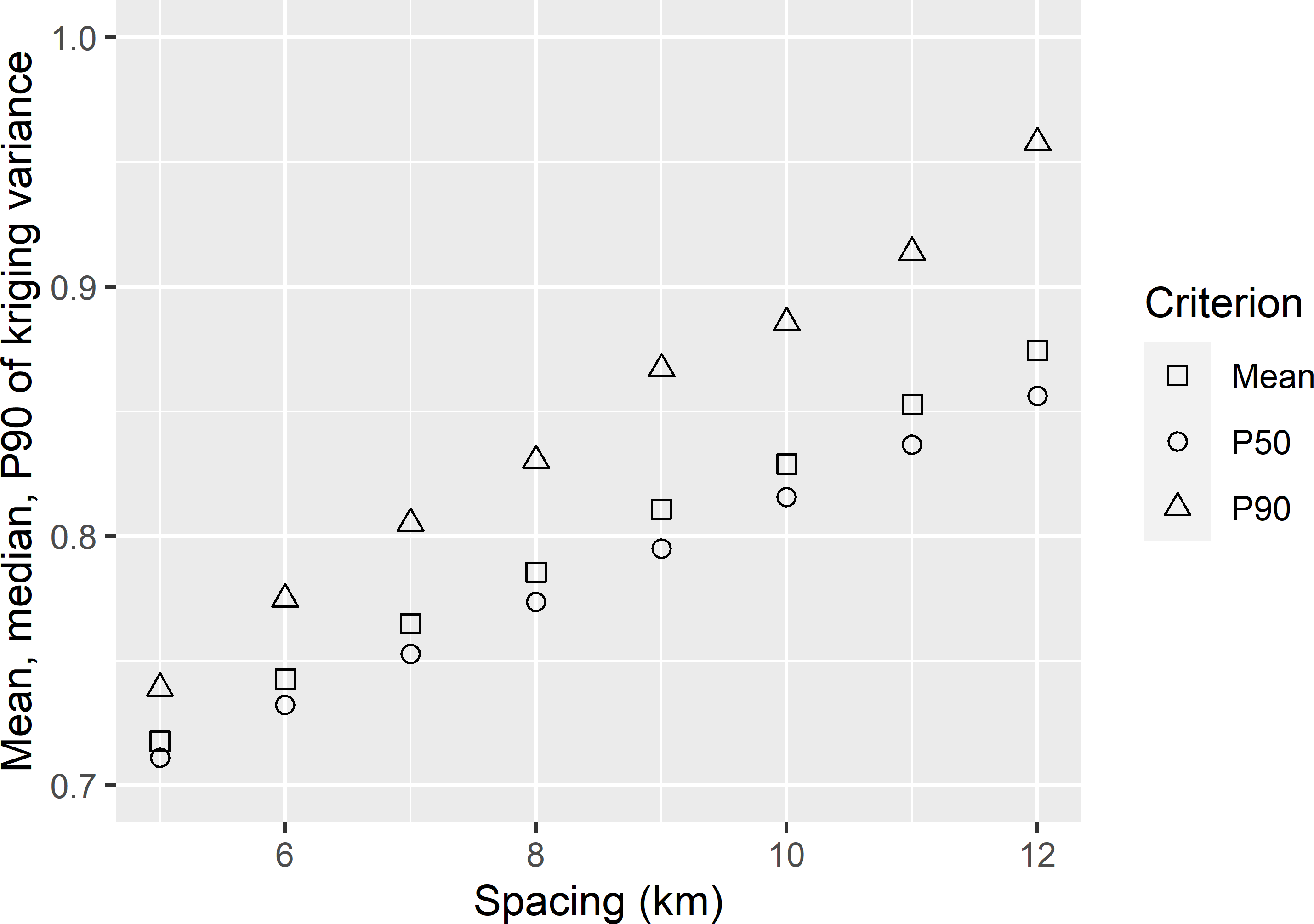
Figure 22.2: Mean, median (P50), and 0.90 quantile (P90) of the ordinary kriging variance of predictions of the SOM concentration in West-Amhara, as a function of the spacing of a square grid.

The tolerable grid spacing for the three quality indices can be computed with function approx of the base package, as shown below for the median kriging variance.

spacing_tol_P50 <- approx(x = dfKV_OK$P50, y = dfKV_OK$spacing, xout = 0.8)$y

For a mean kriging variance of 0.8 (dag kg^-1)² the tolerable grid spacing is 8.6 km. For the median kriging variance this is 9.2 km, which is somewhat larger leading to a smaller sample size. The smaller grid spacing for the mean can be explained by the right-skewed distribution of the kriging variance, so that the mean kriging variance is larger than the median kriging variance. For the P90 of the kriging variance, the tolerable grid spacing is much smaller, 6.8 km, leading to a much larger sample size.

Exercises

1. Write an R script to determine the tolerable grid spacing so that the 0.50, 0.80, and 0.95 quantiles of the variance of OK predictions of SOM in West-Amhara do not exceed 0.85. Estimate the semivariogram by MoM.
   
2. In practice, we are uncertain about the semivariogram. For this reason, it can be wise to explore the sensitivity of the tolerable grid spacing for the semivariogram parameters.
   • Increase the nugget parameter of the MoM semivariogram by 5%, and change the partial sill parameter so that the sill (nugget + partial sill) is unchanged. Compute the tolerable grid spacing and the corresponding required sample size for a mean kriging variance of 0.85 (dag kg^-1)². Explain the difference.
   • Reduce the range of the MoM semivariogram by 5%. Reset the nugget and the partial sill to their original values. Compute the tolerable grid spacing and the corresponding required sample size for a mean kriging variance of 0.85 (dag kg^-1)². Explain the difference.

22.3 Optimal grid spacing for block-kriging

In the previous section, the tolerable grid spacing is derived from a constraint on the mean or quantile of the prediction error variances at points. The alternative is to put a constraint on the mean or quantile of the error variances of the predicted means of blocks. These means can be predicted with block-kriging (Section 21.2). Block-kriging predictions can be obtained with function krige of package gstat using argument block. In the code chunk below, the means of 100 m \(\times\) 100 m blocks are predicted by ordinary block-kriging.

MKV_OBK <- P50KV_OBK <- P90KV_OBK <- numeric(length = length(spacing))
for (i in seq_len(length(spacing))) {
  mygrid <- spsample(x = grdAmhara, cellsize = spacing[i],
    type = "regular", offset = c(0.5, 0.5))
  mygrid$dummy <- rep(1, length(mygrid))
  samplesize[i] <- nrow(mygrid)
  predictions  <- krige(
    formula = dummy ~ 1,
    locations = mygrid,
    newdata = mysample,
    model = vgm_ML_gstat,
    block = c(0.1, 0.1),
    nmax = 100,
    debug.level = 0)
  MKV_OBK[i] <- mean(predictions$var1.var)
  P50KV_OBK[i] <- quantile(predictions$var1.var, probs = 0.5)
  P90KV_OBK[i] <- quantile(predictions$var1.var, probs = 0.9)
}
dfKV_OBK <- data.frame(spacing, MKV_OBK, P50KV_OBK, P90KV_OBK)

Figure 22.3 shows that the mean, P50, and P90 of the block-kriging predictions are substantially smaller than those of the point-kriging predictions (Figure 22.2). This can be explained by the large nugget of the semivariogram (Table 22.1). The side length of a prediction block (100 m) is much smaller than the range of the semivariogram (36.9 km), so that in this case the mean semivariance within a prediction block is about equal to the nugget. Roughly speaking, for a given grid spacing the mean point-kriging variance is reduced by an amount about equal to this mean semivariance to yield the mean block-kriging variance for this spacing (Section 21.2). Recall that the mean semivariance within a block is a model-based prediction of the variance within a block (Subsection 13.1.1, Equation (13.3)).

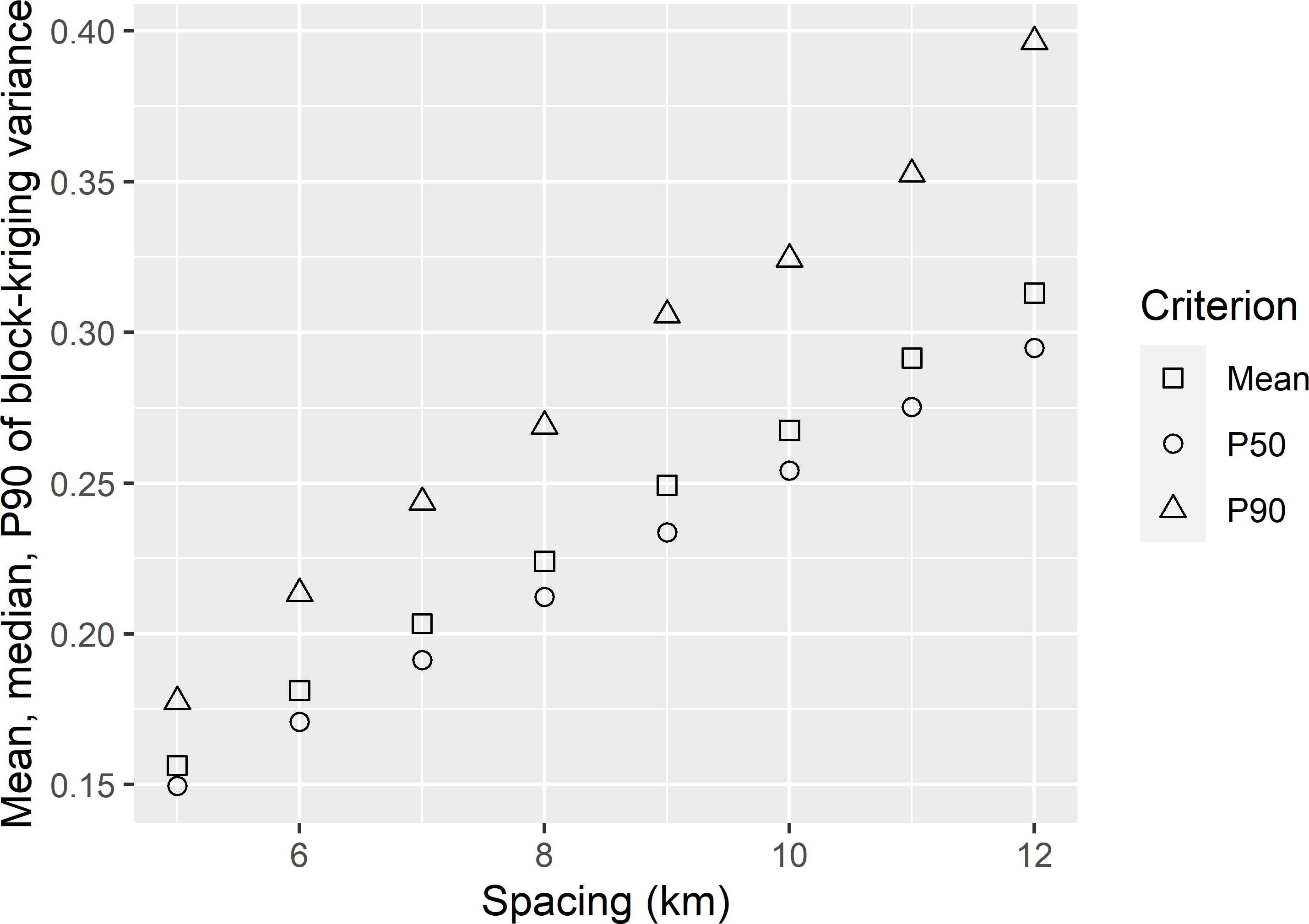
Figure 22.3: Mean, median (P50), and 0.90 quantile (P90) of the ordinary block-kriging variance of predictions of the mean SOM concentration of blocks of 100 m \(\times\) 100 m, in West-Amhara, as a function of the spacing of a square grid.

22.4 Optimal grid spacing for kriging with an external drift

In the previous sections I assumed a constant model-mean for the study variable. I now consider the case where covariates that are related to the study variable are available. A model is calibrated that is the sum of a linear combination of the covariates (spatial trend) and a spatially structured residual, see Equation (21.16). Predictions at the nodes of a fine grid are obtained by kriging with an external drift (KED).

The SOM concentration data of West-Amhara are used to estimate the parameters (regression coefficients and residual semivariogram parameters) of the model by restricted maximum likelihood (REML), see Subsection 21.5.2.

library(geoR)
dGeoR <- as.geodata(obj = sampleAmhara, header = TRUE,
  coords.col = c("s1", "s2"), data.col = "SOM",
  covar.col = c("dem", "rfl_NIR", "rfl_red", "lst"))
vgm_REML <- likfit(geodata = dGeoR, trend = ~ dem + rfl_NIR + rfl_red + lst,
  cov.model = "spherical", ini.cov.pars = c(1, 5),
  nugget = 0.2, lik.method = "REML", messages = FALSE)

Table 22.2: Maximum likelihood (ML) estimates of the parameters of a spherical semivariogram for the SOM concentration and restricted maximum likelihood (REML) estimates of the parameters of a spherical semivariogram for the residuals of a multiple linear regression model, for West-Amhara.

Parameter	ML	REML
nugget	0.56	0.36
partial sill	0.68	0.44
range (km)	36.91	5.24

The total sill (partial sill + nugget) of the residual semivariogram, estimated by REML, equals 0.80, which is considerably smaller than that of the ML semivariogram of SOM (Table 22.2). A considerable part of the variance of SOM is explained by the covariates. Besides, note the much smaller range of the residual semivariogram. The smaller sill and range of the residual semivariogram show that the spatial structure of SOM is largely captured by the covariates. The residuals of the model-mean, which is a linear combination of the covariates, no longer show much spatial structure.

The mean kriging variance as obtained with KED is used as the evaluation criterion. With KED, the kriging variance is also a function of the values of the covariates at the sampling locations and the prediction location (Section 21.3). Compared with the procedure above for OK, in the code chunk below, a slightly different procedure is used. The square grid of a given spacing is randomly placed on the area (option offset in function spsample is not used), and this is repeated ten times.

R <- 10
MKV_KED <- matrix(nrow = length(spacing), ncol = R)
vgm_REML_gstat <- vgm(model = "Sph", nugget = vgm_REML$nugget,
  psill = vgm_REML$sigmasq, range = vgm_REML$phi)
set.seed(314)
for (i in seq_len(length(spacing))) {
  for (j in 1:R) {
    mygrid <- spsample(x = grdAmhara, cellsize = spacing[i], type = "regular")
    mygrid$dummy <- rep(1, length(mygrid))
    mygrd <- data.frame(over(mygrid, grdAmhara), mygrid)
    coordinates(mygrd) <- ~ x1 + x2
    predictions <- krige(
      formula = dummy ~ dem + rfl_NIR + rfl_red + lst,
      locations = mygrd,
      newdata = mysample,
      model = vgm_REML_gstat,
      nmax = 100,
      debug.level = 0)
    MKV_KED[i, j] <- mean(predictions$var1.var)
  }
}
dfKV_KED <- data.frame(spacing, MKV_KED)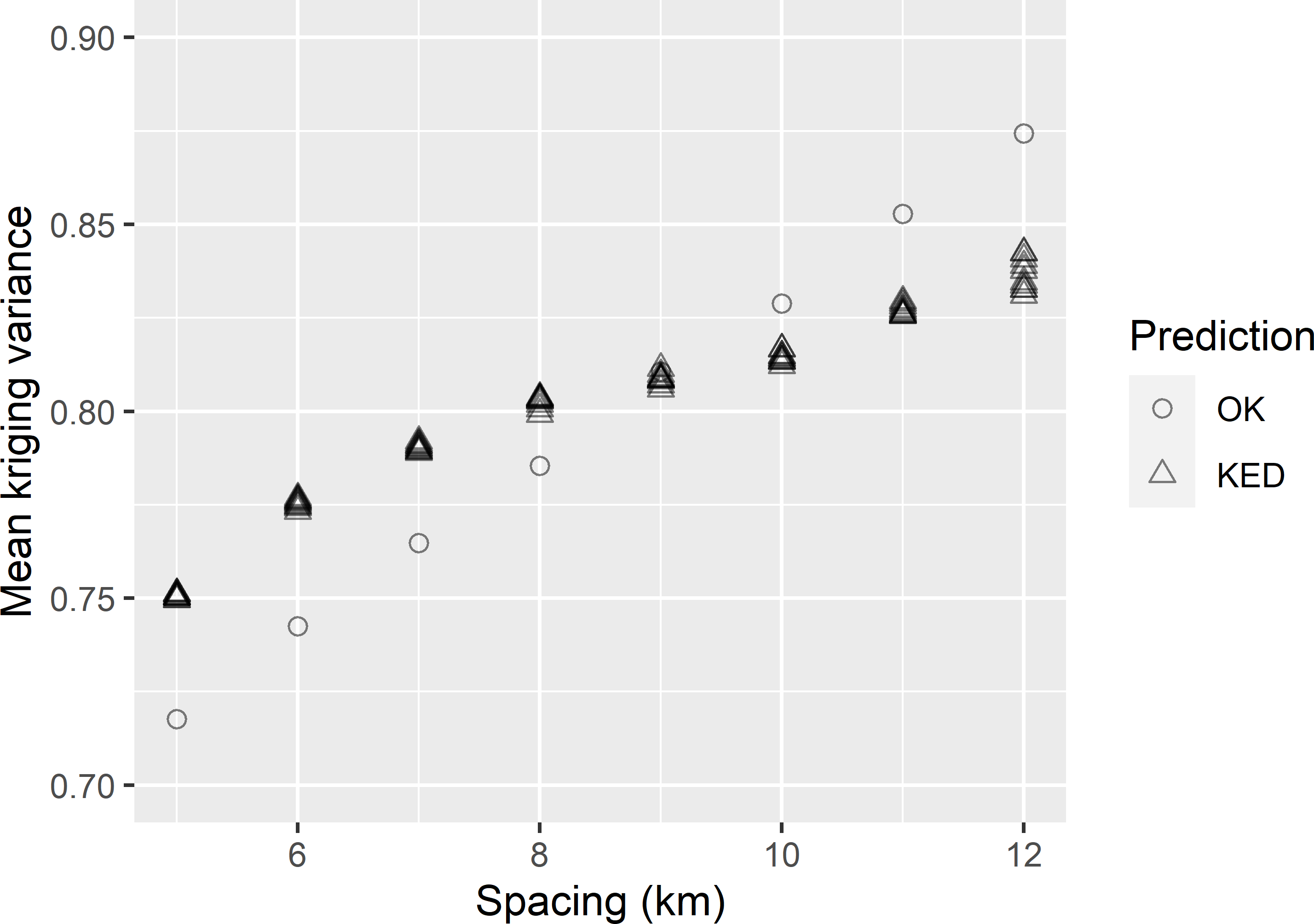

Figure 22.4: Mean kriging variance of OK and KED predictions of the SOM concentration in West-Amhara, as a function of the spacing of a square grid. With KED for each spacing, ten MKV values are shown obtained by selecting ten randomly placed grids of that spacing.

Figure 22.4 shows the mean kriging variances, obtained with OK and KED, as a function of the grid spacing. Interestingly, for grid spacings smaller than about 9 km, the mean kriging variance with KED is larger than with OK. In this case only for larger grid spacings KED outperforms OK in terms of the mean kriging variance. Only for mean kriging variances larger than about 0.82 (dag kg^-1)² we can afford with KED a larger grid spacing (smaller sample size) than with OK. Only with large spacings (small sample sizes) we profit from modelling the mean as a linear function of covariates.

MMKV_KED <- apply(dfKV_KED[, -1], MARGIN = 1, FUN = mean)
spacing_tol_KED <- approx(x = MMKV_KED, y = dfKV_KED$spacing, xout = 0.8)$y

The tolerable grid spacing for a mean kriging variance of 0.8 (dag kg^-1)², using KED, equals 7.9 km.

Exercises

3. Given a grid spacing, the mean kriging variance varies among randomly selected grids, especially for large spacings. Explain why.
   
4. Write an R script to compute the tolerable grid spacing for KED of natural logs of the electrical conductivity of the soil across the Cotton Research Farm of Uzbekistan, using natural logs of the electromagnetic induction (EM) measurements (lnEM100cm) as a covariate. Use a nugget of 0.126, a partial sill of 0.083, and a range of 230 m for an exponential semivariogram of the residuals (Table 23.1). Select a simple random sample of size 1,000 of evaluation points from the discretisation grid with interpolated lnEM100cm values to compute the mean kriging variance. Do this by selecting 1,000 grid cells by simple random sampling with replacement and jittering the centres of the selected grid cells by an amount equal to half the size of the grid cell. Use as grid spacings \(70, 75, \dots, 100\) m. With a spacing of 100 m the number of grid points is about 100 (the farm has an area of about 97 ha). What is the tolerable grid spacing for a mean kriging variance of 0.165?

22.5 Bayesian approach

In practice, we do not know the semivariogram. In the best case we have prior data that can be used to estimate the semivariogram. However, even in this case we are uncertain about the semivariogram model (spherical, exponential, etc.) and the semivariogram parameters. Lark et al. (2017) showed how in a Bayesian approach we can account for uncertainty about the semivariogram parameters when we must decide on the grid spacing. In this approach a prior distribution of the semivariogram parameters is updated with the sample data to a posterior distribution (Gelman et al. 2013):

\[\begin{equation} f(\pmb{\theta}|\mathbf{z}) = \frac{f(\pmb{\theta}) f(\mathbf{z}|\pmb{\theta})} {f(\mathbf{z})}\;, \tag{22.1} \end{equation}\]

with \(f(\pmb{\theta}|\mathbf{z})\) the posterior distribution function, i.e., the probability density function of the semivariogram parameters given the sample data, \(f(\pmb{\theta})\) our prior belief in the parameters specified by a probability density function, \(f(\mathbf{z}|\pmb{\theta})\) the likelihood of the data, and \(f(\mathbf{z})\) the probability density function of the data. This probability density function \(f(\mathbf{z})\) is hard to obtain.

Problems with analytical derivation of the posterior distribution are avoided by selecting a large sample of units (vectors with semivariogram parameters) from the posterior distribution through Markov chain Monte Carlo (MCMC) sampling, see Subsection 13.1.3.

In a Bayesian approach, we must define the likelihood function of the data, see Subsection 13.1.3. I assume that the SOM concentration data in West-Amhara have a multivariate normal distribution, and that the spatial covariance of the data can be modelled by a spherical model, see Subsection 21.4.2. The likelihood is a function of the semivariogram parameters. Given a vector of semivariogram parameters, the variance-covariance matrix of the data is computed from the matrix with geographic distances between the sampling points. Inputs of the log-likelihood function ll are the matrix with distances between the sampling points, the design matrix X, and the vector with observations of the study variable z, see Subsection 13.1.3.

D <- as.matrix(dist(sampleAmhara[,c("s1","s2")]))
X <- matrix(1, nrow(sampleAmhara), 1)
z <- sampleAmhara$SOM

Besides the likelihood function, in a Bayesian approach we must define prior distributions for the semivariogram parameters. Here, we combine the partial sill and nugget into the ratio of spatial dependence, i.e., the proportion of the sill attributable to the partial sill. For the ratio of spatial dependence \(\xi\) and the distance parameter \(\phi\), I use uniform distributions as priors, with a lower bound of 0 and an upper bound of 1 for the ratio of spatial dependence, and a lower bound of \(10^{-6}\) km and an upper bound of 100 km for the range. A uniform distribution for the sill is not recommended (Gelman et al. 2013). Instead, I assume a uniform distribution for the inverse of the sill, with a lower bound of \(10^{-6}\) and an upper bound of 2.

These priors can be defined by function createUniformPrior of package BayesianTools (Hartig, Minunno, and Paul 2019). There are also functions to define a beta density function (commonly used as a prior for proportions) and a truncated normal distribution as a prior. Function createBayesianSetup is then used to define the setup of the MCMC sampling, specifying the likelihood function, the prior, and the vector with best prior estimates of the model parameters, specified with argument best. The ML estimates computed in Section 22.1 are used as starting values for the inverse of the sill parameter, the ratio of spatial dependence, and the range.

library(BayesianTools)
priors <- createUniformPrior(
  lower = c(1E-6, 0, 1E-6), upper = c(2, 1, 100))
sill_ML <- vgm_ML$nugget + vgm_ML$sigmasq
thetas_ML <- c(1 / sill_ML, vgm_ML$sigmasq / sill_ML, vgm_ML$phi)
model <- "Sph"
setup <- createBayesianSetup(likelihood = ll, prior = priors,
  best = thetas_ML, names = c("lambda", "xi", "range"))

A sample from the posterior distribution of the semivariogram parameters is then obtained with function runMCMC. Various sampling algorithms are implemented in package BayesianTools. I used the default sampler DEzs, which is based on the differential evolution Markov chain (ter Braak and Vrugt 2008). This algorithm is passed to function runMCMC with argument sampler. It is common not to use all sampled units, but to discard the units of the burn-in period that are possibly influenced by the initial arbitrary settings, and to thin the series of units after this period. The extraction of the ultimate sample is done with function getSample. Argument start specifies the unit where the extraction starts, and argument numSamples specifies how many units are selected through systematic sampling of the full MCMC sample. The alternative is to use argument thin which defines the thinning interval.

set.seed(314)
res <- runMCMC(setup, sampler = "DEzs")
mcmcsample <- getSample(res, start = 1000, numSamples = 1000) %>%
  data.frame()

Table 22.3 shows the first ten units of the MCMC sample from the posterior distribution of the semivariogram parameters.

Table 22.3: First ten units of a MCMC sample from the posterior distribution of the parameters of a spherical semivariogram for the SOM concentration in West-Amhara.

Inverse of sill	Ratio of spatial dependence	Range (km)
0.624	0.655	55.0
0.828	0.588	33.3
0.769	0.480	51.9
0.624	0.655	55.0
0.872	0.538	47.2
0.559	0.643	60.6
0.605	0.690	66.8
0.764	0.585	42.7
0.793	0.608	44.8
0.480	0.741	87.1

The units of the MCMC sample (vectors with semivariogram parameters) are used one-by-one to compute the average of the kriging variances at the simple random sample of evaluation points.

For each unit in the MCMC sample, the tolerable grid spacing is computed for a target MKV of 0.8. Figure 22.5 shows that for most sampled semivariograms (MCMC sample units) the tolerable grid spacing equals 8 km, which roughly corresponds with the tolerable grid spacing derived above for OK. For 165 sampled semivariograms, the tolerable grid spacing exceeds 12 km. However, this grid spacing leads to a sample size that is too small for estimating the semivariogram and kriging.

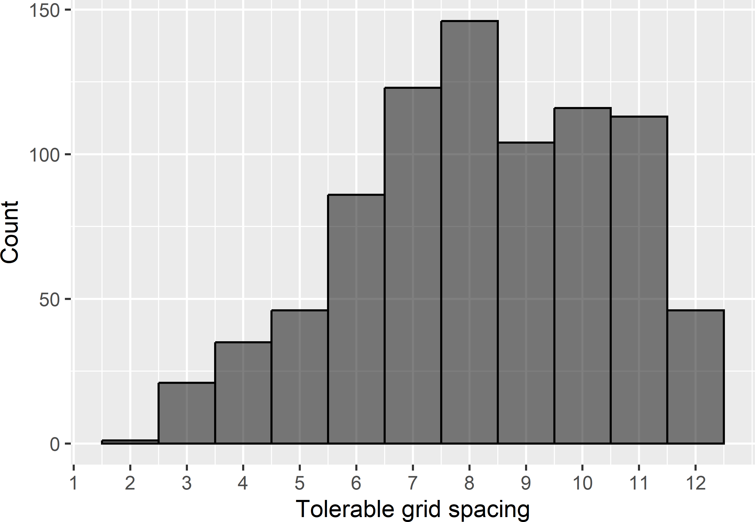
Figure 22.5: Frequency distribution of tolerable grid spacings for a target MKV of 0.8.

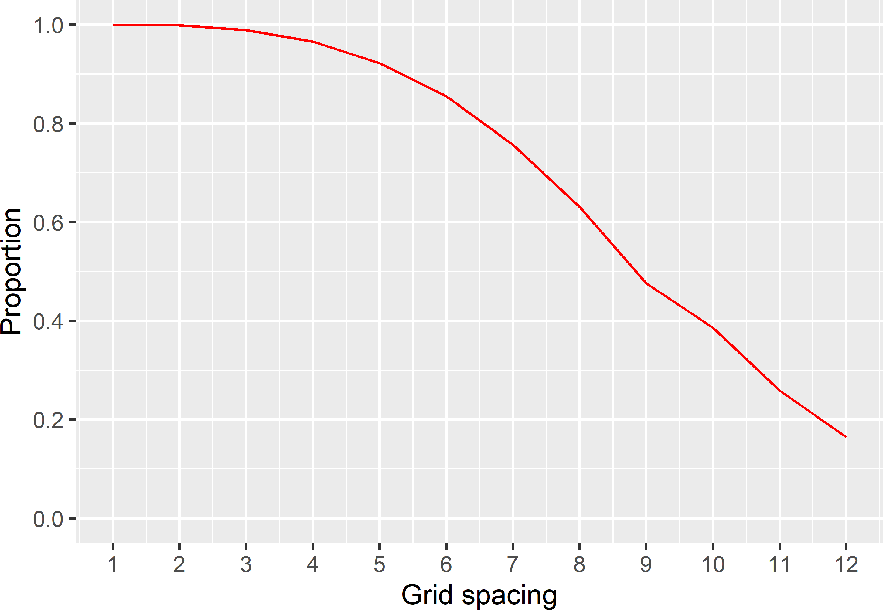
Figure 22.6: Proportion of sampled semivariograms with a MKV smaller than or equal to a target MKV of 0.8.

Finally, for each grid spacing, the proportion of MCMC samples with a MKV smaller than or equal to the target MKV of 0.8 is computed. Figure 22.6 shows, for instance, that if the MKV is required not to exceed a target MKV of 0.8 with a probability of 80%, the tolerable grid spacing is 6.6 km. With a grid spacing of 8.6 km, as determined before, the probability that the MKV exceeds 0.8 is 54%.

References

Gelman, A., J. B. Carlin, H. S. Stern, D. B. Dunson, A. Vehtari, and D. B. Rubin. 2013. Bayesian Data Analysis. Third. Boca Raton: Chapman & Hall/CRC.

Hartig, F., F. Minunno, and S. Paul. 2019. BayesianTools: General-Purpose MCMC and SMC Samplers and Tools for Bayesian Statistics. https://CRAN.R-project.org/package=BayesianTools.

Lark, R. M., E. M. Hamilton, B. Kaninga, K. K. Maseka, M. Mutondo, G. M. Sakala, and M. J. Watts. 2017. “Planning Spatial Sampling of the Soil from an Uncertain Reconnaissance Variogram.” SOIL 3 (4): 235–44.

Pebesma, E. J. 2004. “Multivariable Geostatistics in S: The Gstat Package.” Computers & Geosciences 30 (7): 683–91.

Ribeiro Jr, Paulo J., Peter J. Diggle, Martin Schlather, Roger Bivand, and Brian Ripley. 2020. geoR: Analysis of Geostatistical Data. https://CRAN.R-project.org/package=geoR.

ter Braak, C. J. F., and J. A. Vrugt. 2008. “Differential Evolution Markov Chain with snooker updater and fewer chains.” Statistics and Computing 18 (4): 435–46. https://doi.org/DOI 10.1007/s11222-008-9104-9.

---

12. Spatial response surface sampling can also be considered as model-based sampling, especially when a model-based criterion is used, see Chapter 20.↩︎

13. This is mainly done to avoid problems in (restricted) maximum likelihood estimation of the (residual) semivariogram with function likfit of package geoR.↩︎