Chapter 4 Stratified simple random sampling
In stratified random sampling the population is divided into subpopulations, for instance, soil mapping units, areas with the same land use or land cover, administrative units, etc. The subareas are mutually exclusive, i.e., they do not overlap, and are jointly exhaustive, i.e., their union equals the entire population (study area). Within each subpopulation, referred to as a stratum, a probability sample is selected by some sampling design. If these probability samples are selected by simple random sampling, as described in the previous chapter, the design is stratified simple random sampling, the topic of this chapter. If sampling units are selected by cluster random sampling, then the design is stratified cluster random sampling.
Stratified simple random sampling is illustrated with Voorst (Figure 4.1). Tibble grdVoorst with simulated data contains variable stratum. The strata are combinations of soil class and land use, obtained by overlaying a soil map and a land use map. To select a stratified simple random sample, we set the total sample size \(n\). The sampling units must be apportioned to the strata. I chose to apportion the units proportionally to the size (area, number of grid cells) of the strata (for details, see Section 4.3). The larger a stratum, the more units are selected from this stratum. The sizes of the strata, i.e., the total number of grid cells, are computed with function tapply.
N_h <- tapply(grdVoorst$stratum, INDEX = grdVoorst$stratum, FUN = length)
w_h <- N_h / sum(N_h)
n <- 40
print(n_h <- round(n * w_h))
BA EA PA RA XF
13 8 9 4 7 The sum of the stratum sample sizes is 41; we want 40, so we reduce the largest stratum sample size by 1.
The stratified simple random sample is selected with function strata of package sampling (Tillé and Matei 2021). Argument size specifies the stratum sample sizes.
grdVoorst, which is determined first with function unique.
Within the strata, the grid cells are selected by simple random sampling with replacement (method = "srswr"), so that in principle more than one point can be selected within a grid cell, see Chapter 3 for a motivation of this. Function getdata extracts the observations of the selected units from the sampling frame, as well as the spatial coordinates and the stratum of these units. The coordinates of the centres of the selected grid cells are jittered by an amount equal to half the side of the grid cells. In the next code chunk, this is done with function mutate of package dplyr (Hadley Wickham et al. 2021) which is part of package tidyverse (Hadley Wickham et al. 2019). We have seen the pipe operator %>% of package magrittr (Bache and Wickham 2020) before in Subsection 3.1.2. If you are not familiar with tidyverse I recommend reading the excellent book (H. Wickham and Grolemund 2017).
library(sampling)
ord <- unique(grdVoorst$stratum)
set.seed(314)
units <- sampling::strata(
  grdVoorst, stratanames = "stratum", size = n_h[ord], method = "srswr")
mysample <- getdata(grdVoorst, units) %>%
  mutate(s1 = s1 %>% jitter(amount = 25 / 2),
s2 = s2 %>% jitter(amount = 25 / 2))strata (sampling::strata), as strata is also a function of another package. Not adding the name of the package may result in an error message.
Figure 4.1 shows the selected sample.
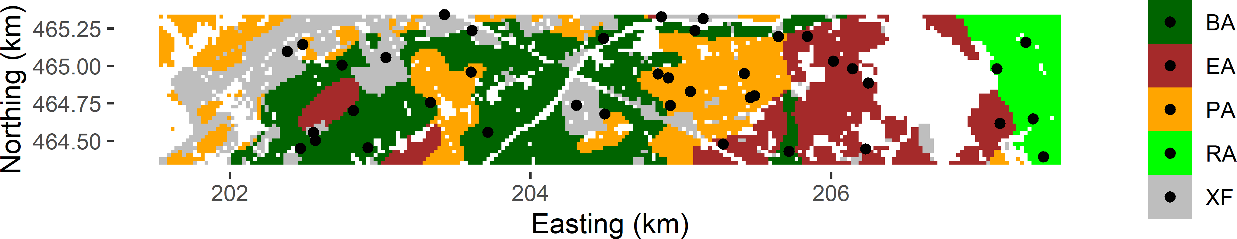
Figure 4.1: Stratified simple random sample of size 40 from Voorst. Strata are combinations of soil class and land use.
4.1 Estimation of population parameters
With simple random sampling within strata, the estimator of the population mean for simple random sampling (Equation (3.2)) is applied at the level of the strata. The estimated stratum means are then averaged, using the relative sizes or areas of the strata as weights:
\[\begin{equation} \hat{\bar{z}}= \sum\limits_{h=1}^{H} w_{h}\,\hat{\bar{z}}_{h} \;, \tag{4.1} \end{equation}\]
where \(H\) is the number of strata, \(w_{h}\) is the relative size (area) of stratum \(h\) (stratum weight): \(w_h = N_h/N\), and \(\hat{\bar{z}}_{h}\) is the estimated mean of stratum \(h\), estimated by the sample mean for stratum \(h\):
\[\begin{equation} \hat{\bar{z}}_{h}=\frac{1}{n_h}\sum_{k \in \mathcal{S}_h} z_k\;, \tag{4.2} \end{equation}\]
with \(\mathcal{S}_h\) the sample selected from stratum \(h\).
The same estimator is found when the \(\pi\) estimator is worked out for stratified simple random sampling. With stratified simple random sampling without replacement and different sampling fractions for the strata, the inclusion probabilities differ among the strata and equal \(\pi_{k} = n_h/N_h\) for all \(k\) in stratum \(h\), with \(n_h\) the sample size of stratum \(h\) and \(N_h\) the size of stratum \(h\). Inserting this in the \(\pi\) estimator of the population mean (Equation (2.4)) gives
\[\begin{equation} \hat{\bar{z}}= \frac{1}{N}\sum\limits_{h=1}^{H}\sum\limits_{k \in \mathcal{S}_h} \frac{z_{k}}{\pi_{k}} = \frac{1}{N}\sum\limits_{h=1}^{H} \frac{N_h}{n_h}\sum\limits_{k \in \mathcal{S}_h} z_{k} = \sum\limits_{h=1}^{H} w_{h}\,\hat{\bar{z}}_{h} \;. \tag{4.3} \end{equation}\]
The sampling variance of the estimator of the population mean is estimated by first estimating the sampling variances of the estimated stratum means, followed by computing the weighted average of the estimated sampling variances of the estimated stratum means. Note that we must square the stratum weights:
\[\begin{equation} \widehat{V}\!\left(\hat{\bar{z}}\right)=\sum\limits_{h=1}^{H}w_{h}^{2}\,\widehat{V}\!\left(\hat{\bar{z}}_{h}\right)\;, \tag{4.4} \end{equation}\]
where \(\widehat{V}\!\left(\hat{\bar{z}}_{h}\right)\) is the estimated sampling variance of \(\hat{\bar{z}}_{h}\):
\[\begin{equation} \widehat{V}\!\left(\hat{\bar{z}}_{h}\right)= (1-\frac{n_h}{N_h}) \frac{\widehat{S^2}_h(z)}{n_h}\;, \tag{4.5} \end{equation}\]
with \(\widehat{S^2}_h(z)\) the estimated variance of \(z\) within stratum \(h\):
\[\begin{equation} \widehat{S^2}_h(z)=\frac{1}{n_h-1}\sum\limits_{k \in \mathcal{S}_h}\left(z_{k}-\hat{\bar{z}}_{h}\right)^{2}\;. \tag{4.6} \end{equation}\]
For stratified simple random sampling with replacement of finite populations and stratified simple random sampling of infinite populations the fpcs \(1-(n_h/N_h)\) can be dropped.
mz_h <- tapply(mysample$z, INDEX = mysample$stratum, FUN = mean)
mz <- sum(w_h * mz_h)
S2z_h <- tapply(mysample$z, INDEX = mysample$stratum, FUN = var)
v_mz_h <- S2z_h / n_h
se_mz <- sqrt(sum(w_h^2 * v_mz_h))| Stratum | Nh | nh | Mean | Variance | se |
|---|---|---|---|---|---|
| BA | 2,371 | 12 | 91.1 | 946.3 | 8.9 |
| EA | 1,442 | 8 | 58.3 | 555.5 | 8.3 |
| PA | 1,710 | 9 | 59.4 | 214.7 | 4.9 |
| RA | 659 | 4 | 103.2 | 2,528.8 | 25.1 |
| XF | 1,346 | 7 | 133.9 | 3,807.3 | 23.3 |
Table 4.1 shows per stratum the estimated mean, variance, and sampling variance of the estimated mean of the SOM concentration. We can see large differences in the within-stratum variances. For the stratified sample of Figure 4.1, the estimated population mean equals 86.3 g kg-1, and the estimated standard error of this estimator equals 5.8 g kg-1.
The population mean can also be estimated directly using the basic \(\pi\) estimator (Equation (2.4)). The inclusion probabilities are included in data.frame mysample, obtained with function getdata (see code chunk above), as variable Prob.
           s1       s2         z stratum ID_unit        Prob Stratum
1135 202554.8 464556.7 186.99296      XF    1135 0.005189017       1
2159 204305.5 464738.9  75.04809      XF    2159 0.005189017       1
4205 203038.3 465057.0 138.14617      XF    4205 0.005189017       1
4503 202381.1 465096.7  69.43803      XF    4503 0.005189017       1
5336 203610.4 465237.8  78.02003      XF    5336 0.005189017       1
5853 205147.1 465315.5 164.55224      XF    5853 0.005189017       1
The population total is estimated first, and by dividing this estimated total by the total number of population units \(N\) an estimate of the population mean is obtained.
[1] 86.53333The two estimates of the population mean are not exactly equal. This is due to rounding errors in the inclusion probabilities. This can be shown by computing the sum of the inclusion probabilities over all population units. This sum should be equal to the sample size \(n=40\), but as we can see below, this sum is slightly smaller.
[1] 39.90711Now suppose we ignore that the sample data come from a stratified sampling design and we use the (unweighted) sample mean as an estimate of the population mean.
[1] 86.11247The sample mean slightly differs from the proper estimate of the population mean (86.334). The sample mean is a biased estimator, but the bias is small. The bias is only small because the stratum sample sizes are about proportional to the sizes of the strata, so that the inclusion probabilities (sampling intensities) are about equal for all strata: 0.0050494, 0.0055344, 0.0052509, 0.006056, 0.005189. The probabilities are not exactly equal because the stratum sample sizes are necessarily rounded to integers and because we reduced the largest sample size by one unit. The bias would have been substantially larger if an equal number of units would have been selected from each stratum, leading to much larger differences in the inclusion probabilities among the strata. Sampling intensity in stratum BA, for instance, then would be much smaller compared to the other strata, and so would be the inclusion probabilities of the units in this stratum as compared to the other strata. Stratum BA then would be underrepresented in the sample. This is not a problem as long as we account for the difference in inclusion probabilities of the units in the estimation of the population mean. The estimated mean of stratum BA then gets the largest weight, equal to the inverse of the inclusion probability. If we do not account for these differences in inclusion probabilities, the estimator of the mean will be seriously biased.
The next code chunk shows how the population mean and its standard error can be estimated with package survey (Lumley 2021). Note that the stratum weights \(N_h/n_h\) must be passed to function svydesign using argument weight. These are first attached to data.frame mysample by creating a look-up table lut, which is then merged with function merge to data.frame mysample.
library(survey)
labels <- sort(unique(mysample$stratum))
lut <- data.frame(stratum = labels, weight = N_h / n_h)
mysample <- merge(x = mysample, y = lut)
design_stsi <- svydesign(
  id = ~ 1, strata = ~ stratum, weight = ~ weight, data = mysample)
svymean(~ z, design_stsi)
mean SE
z 86.334 5.81674.1.1 Population proportion, cumulative distribution function, and quantiles
The proportion of a population satisfying some condition can be estimated by Equations (4.1) and (4.2), substituting for the study variable \(z_k\) an 0/1 indicator \(y_k\) with value 1 if for unit \(k\) the condition is satisfied, and 0 otherwise (Subsection 3.1.1). In general, with stratified simple random sampling the inclusion probabilities are not exactly equal, so that the estimated population proportion is not equal to the sample proportion.
These unequal inclusion probabilities must also be accounted for when estimating the cumulative distribution function (CDF) and quantiles (Subsection 3.1.2), as shown in the next code chunk for the CDF.
thresholds <- sort(unique(mysample$z))
cumfreq <- numeric(length = length(thresholds))
for (i in seq_len(length(thresholds))) {
  ind <- mysample$z <= thresholds[i]
  mh_ind <- tapply(ind, INDEX = mysample$stratum, FUN = mean)
  cumfreq[i] <- sum(w_h * mh_ind)
}
df <- data.frame(x = thresholds, y = cumfreq)
Figure 4.2 shows the estimated CDF, estimated from the stratified simple random sample of 40 units from Voorst (Figure 4.1).
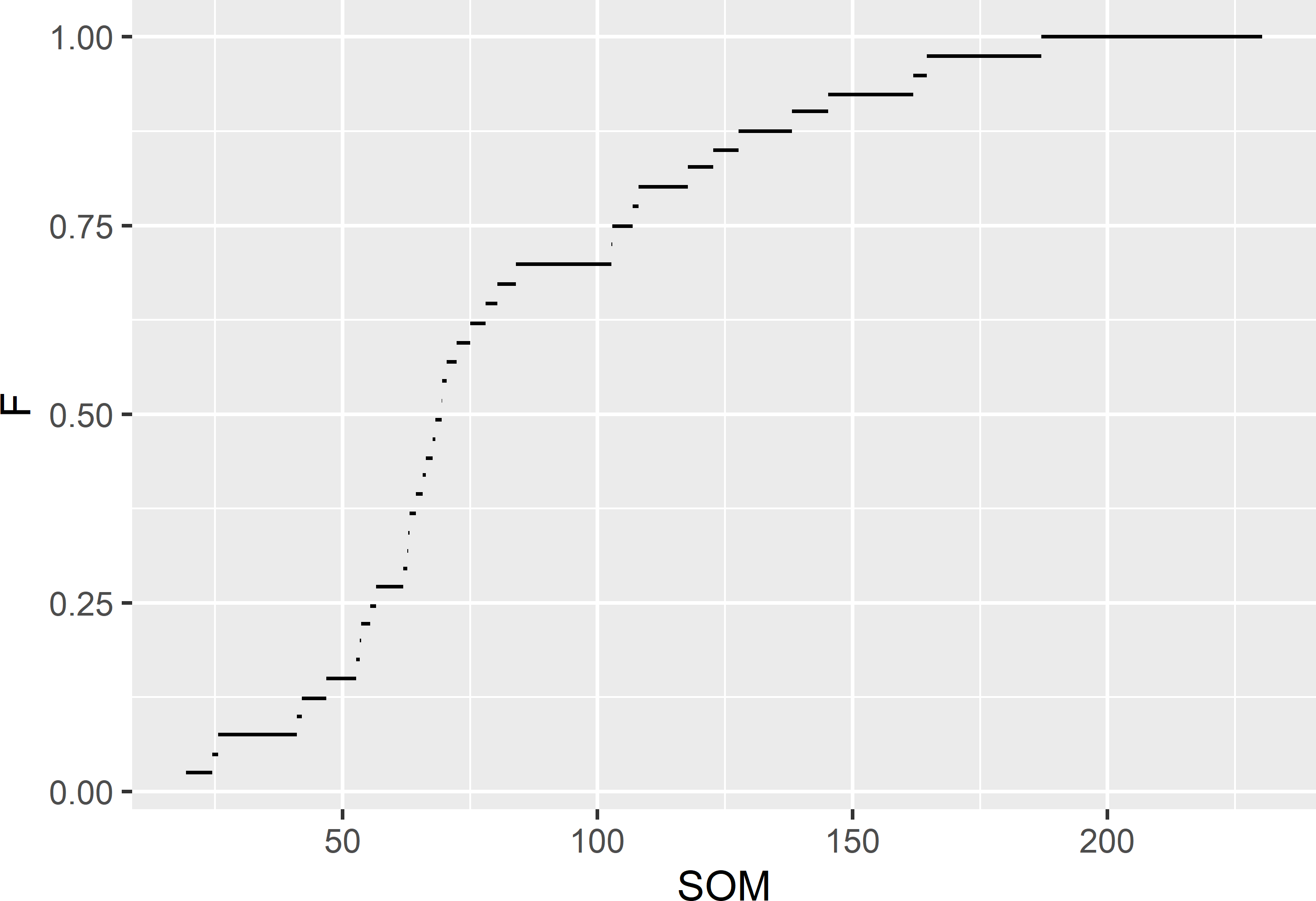
Figure 4.2: Estimated cumulative distribution function of the SOM concentration (g kg-1) in Voorst, estimated from the stratified simple random sample of 40 units.
The estimated proportions, or cumulative frequencies, are used to estimate a quantile. These estimates are easily obtained with function svyquantile of package survey.
$z
     quantile    ci.2.5   ci.97.5        se
0.5  69.56081  65.70434  84.03993  4.515916
0.8 117.73877 102.75359 161.88611 14.563887

attr(,"hasci")
[1] TRUE
attr(,"class")
[1] "newsvyquantile"
4.1.2 Why should we stratify?
There can be two reasons for stratifying the population:
- we are interested in the mean or total per stratum; or
- we want to increase the precision of the estimated mean or total for the entire population.
Figure 4.3 shows boxplots of the approximated sampling distributions of the \(\pi\) estimator of the mean SOM concentration for stratified simple random sampling and simple random sampling, both of size 40, obtained by repeating the random sampling with each design and estimation 10,000 times.
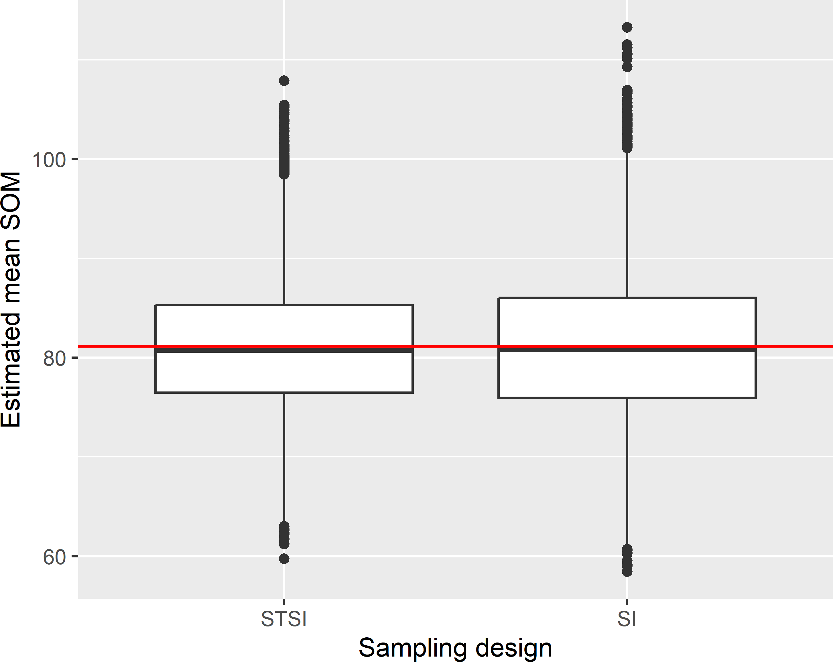
Figure 4.3: Approximated sampling distribution of the \(\pi\) estimator of the mean SOM concentration (g kg-1) in Voorst for stratified simple random sampling (STSI) and simple random sampling (SI) of size 40.
The approximated sampling distributions of the estimators of the population mean with the two designs are not very different. With stratified random sampling, the spread of the estimated means is somewhat smaller. The horizontal red line is the population mean (81.1 g kg-1). The gain in precision due to the stratification, referred to as the stratification effect, can be quantified by the ratio of the variance with simple random sampling and the variance with stratified simple random sampling. So, when this variance ratio is larger than 1, stratified simple random sampling is more precise than simple random sampling. For Voorst the stratification effect with proportional allocation (Section 4.3) equals 1.310. This means that with simple random sampling we need 1.310 more sampling units than with stratified simple random sampling to obtain an estimate of the same precision.
The stratification effect can be computed from the population variance \(S^2(z)\) (Equation (3.8)) and the variances within the strata \(S^2_h(z)\). In the sampling experiment, these variances are known without error because we know the \(z\)-values for all units in the population. In practice, we only know the \(z\)-values for the sampled units. However, a design-unbiased estimator of the population variance is (de Gruijter et al. 2006)
\[\begin{equation} \widehat{S^{2}}(z)= \widehat{\overline{z^{2}}}-\left(\hat{\bar{z}}\right)^{2}+ \widehat{V}\!\left(\hat{\bar{z}}\right) \;, \tag{4.7} \end{equation}\]
where \(\widehat{\overline{z^{2}}}\) denotes the estimated population mean of the study variable squared (\(z^2\)), obtained in the same way as \(\hat{\bar{z}}\) (Equation (4.1)), but using squared values, and \(\widehat{V}\!\left(\hat{\bar{z}}\right)\) denotes the estimated variance of the estimator of the population mean (Equation (4.4)).
The estimated population variance is then divided by the sum of the stratum sample sizes to get an estimate of the sampling variance of the estimator of the mean with simple random sampling of an equal number of units:
\[\begin{equation} \widehat{V}(\hat{\bar{z}}_{\text{SI}}) = \frac{\widehat{S^2}(z)}{\sum_{h=1}^{H}n_h}\;. \tag{4.8} \end{equation}\]
The population variance can be estimated with function s2 of package surveyplanning (Breidaks, Liberts, and Jukams 2020). However, this function is an implementation of an alternative, consistent estimator of the population variance (Särndal, Swensson, and Wretman 1992):
\[\begin{equation} \widehat{S^2}(z) = \frac{N-1}{N} \frac{n}{n-1} \frac{1}{N-1} \sum_{k \in \mathcal{S}} \frac{(z_k - \hat{\bar{z}}_{\pi})^2}{\pi_k} \;. \tag{4.9} \end{equation}\]
The design effect is defined as the variance of an estimator of the population mean with the sampling design under study divided by the variance of the \(\pi\) estimator of the mean with simple random sampling of an equal number of units (Section 12.4). So, the design effect of stratified random sampling is the reciprocal of the stratification effect. For the stratified simple random sample of Figure 4.1, the design effect can then be estimated as follows. Function SE extracts the estimated standard error of the estimator of the mean from the output of function svymean. The extracted standard error is then squared to obtain an estimate of the sampling variance of the estimator of the population with stratified simple random sampling. Finally, this variance is divided by the variance with simple random sampling of an equal number of units.
          z
z 0.6903965
The same value is obtained with argument deff of function svymean.
design_stsi <- svydesign(
  id = ~ 1, strata = ~ stratum, weight = ~ weight, data = mysample)
svymean(~ z, design_stsi, deff = "replace")
mean SE DEff
z 86.3340 5.8167 0.6904So, when using package survey, estimation of the population variance is not needed to estimate the design effect. I only added this to make clear how the design effect is computed with functions in package survey. In following chapters I will skip the estimation of the population variance.
The estimated design effect as estimated from the stratified sample is smaller than 1, showing that stratified simple random sampling is more efficient than simple random sampling. The reciprocal of the estimated design effect (1.448) is somewhat larger than the stratification effect as computed in the sampling experiment, but this is an estimate of the design effect from one stratified sample only. The estimated population variance varies among stratified samples, and so does the estimated design effect.
Stratified simple random sampling with proportional allocation (Section 4.3) is more precise than simple random sampling when the sum of squares of the stratum means is larger than the sum of squares within strata (Lohr 1999):
\[\begin{equation} SSB > SSW\;, \tag{4.10} \end{equation}\]
with SSB the weighted sum-of-squares between the stratum means:
\[\begin{equation} SSB = \sum_{h=1}^H N_h (\bar{z}_h-\bar{z})^2 \;, \tag{4.11} \end{equation}\]
and SSW the sum over the strata of the weighted variances within strata (weights equal to \(1-N_h/N\)):
\[\begin{equation} SSW = \sum_{h=1}^H (1-\frac{N_h}{N})S^2_h\;. \tag{4.12} \end{equation}\]
In other words, the smaller the differences in the stratum means and the larger the variances within the strata, the smaller the stratification effect will be. Figure 4.4 shows a boxplot of the SOM concentration per stratum (soil-land use combination). The stratum means are equal to 83.0, 49.0, 68.8, 92.7, 122.3 g kg-1. The stratum variances are 1799.2, 238.4, 1652.9, 1905.4, 2942.8 (g kg-1)2. The large stratum variances explain the modest gain in precision realised by stratified simple random sampling compared to simple random sampling in this case.
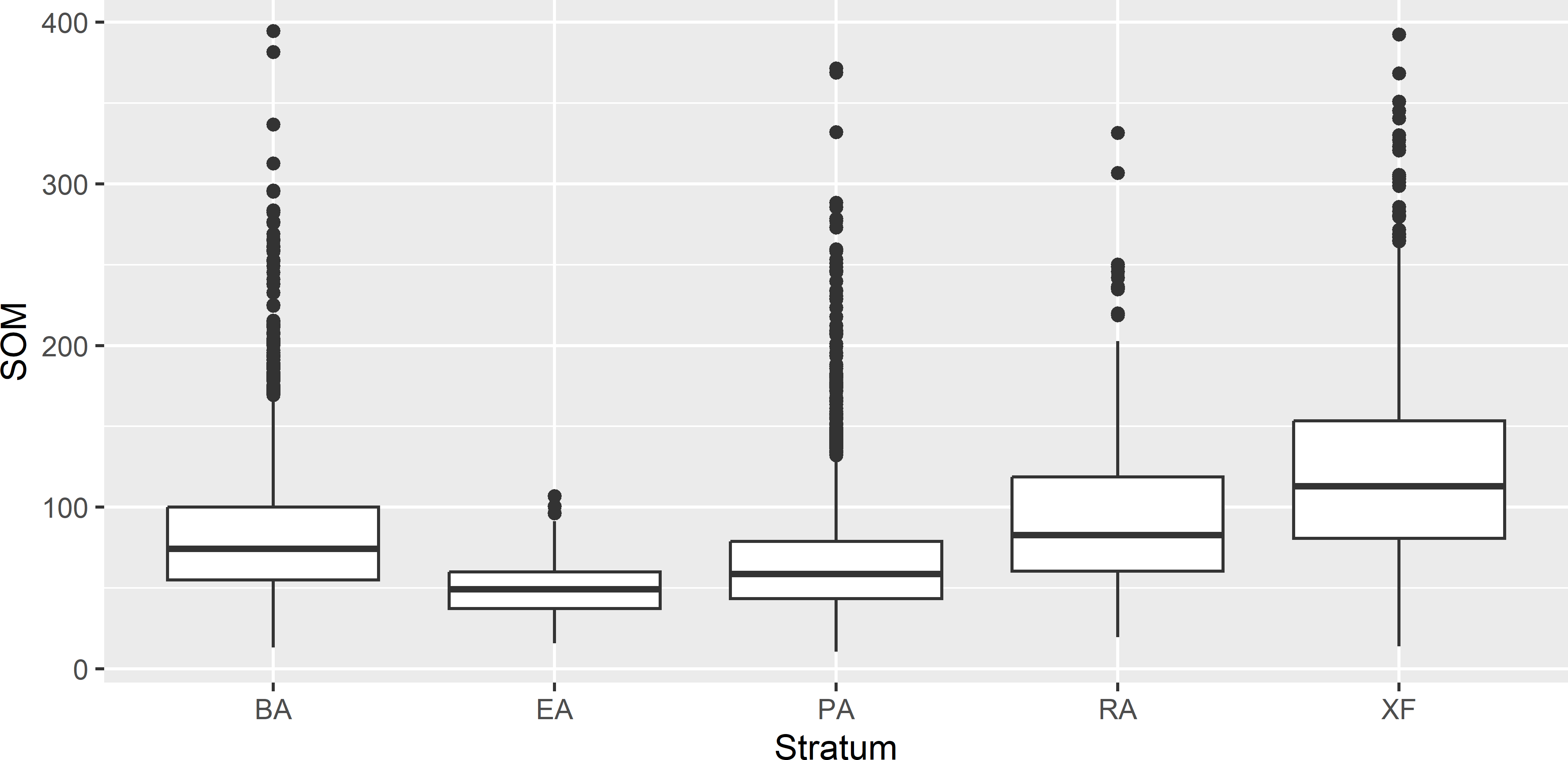
Figure 4.4: Boxplots of the SOM concentration (g kg-1) for the five strata (soil-land use combinations) in Voorst.
4.2 Confidence interval estimate
The \(100(1-\alpha)\)% confidence interval for \(\bar{z}\) is given by
\[\begin{equation} \hat{\bar{z}} \pm t_{\alpha /2, df}\cdot \sqrt{\widehat{V}\!\left(\hat{\bar{z}}\right)} \;, \tag{4.13} \end{equation}\]
where \(t_{\alpha /2,df}\) is the \((1-\alpha /2)\) quantile of a t distribution with \(df\) degrees of freedom. The degrees of freedom \(df\) can be approximated by \(n-H\), as proposed by Lohr (1999). This is the number of the degrees of freedom if the variances within the strata are equal. With unequal variances within strata, \(df\) can be approximated by Sattherwaite’s method (Nanthakumar and Selvavel 2004):
\[\begin{equation} df \approx \frac {\left(\sum_{h=1}^H w_h^2 \frac{\widehat{S^2}_h(z)}{n_h}\right)^2} {\sum_{h=1}^H w_h^4 \left(\frac{\widehat{S^2}_h(z)}{n_h}\right)^2 \frac {1}{n_h-1}} \;. \tag{4.14} \end{equation}\]
A confidence interval estimate of the population mean can be extracted with method confint of package survey. It uses \(n-H\) degrees of freedom.
res <- svymean(~ z, design_stsi)
df_stsi <- degf(design_stsi)
confint(res, df = df_stsi, level = 0.95)
2.5 % 97.5 %
z 74.52542 98.142524.3 Allocation of sample size to strata
After we have decided on the total sample size \(n\), we must decide how to apportion the units to the strata. It is reasonable to allocate more sampling units to large strata and fewer to small strata. The simplest way to achieve this is proportional allocation:
\[\begin{equation} n_{h}=n \cdot \frac{N_{h}}{\sum N_{h}}\;, \tag{4.15} \end{equation}\]
with \(N_h\) the total number of population units (size) of stratum \(h\). With infinite populations \(N_h\) is replaced by the area \(A_h\). The sample sizes computed with this equation are rounded to the nearest integers.
If we have prior information on the variance of the study variable within the strata, then it makes sense to account for differences in variance. Heterogeneous strata should receive more sampling units than homogeneous strata, leading to Neyman allocation:
\[\begin{equation} n_{h}= n \cdot \frac{N_{h}\,S_{h}(z)}{\sum\limits_{h=1}^{H} N_{h}\,S_{h}(z)} \;, \tag{4.16} \end{equation}\]
with \(S_h(z)\) the standard deviation (square root of variance) of the study variable \(z\) in stratum \(h\).
Finally, the costs of sampling may differ among the strata. It can be relatively expensive to sample nearly inaccessible strata, and we do not want to sample many units there. This leads to optimal allocation:
\[\begin{equation} n_{h}= n \cdot \frac{\frac{N_{h}\,S_{h}(z)}{\sqrt{c_{h}}}}{\sum\limits_{h=1}^{H} \frac{N_{h}\,S_{h}(z)}{\sqrt{c_{h}}}} \;, \tag{4.17} \end{equation}\]
with \(c_h\) the costs per sampling unit in stratum \(h\). Optimal means that given the total costs this allocation type leads to minimum sampling variance, assuming a linear costs model:
\[\begin{equation} C = c_0 + \sum_{h=1}^H n_h c_h \;, \tag{4.18} \end{equation}\]
with \(c_0\) overhead costs. So, the more variable a stratum and the lower the costs, the more units will be selected from this stratum.
S2z_h <- tapply(X = grdVoorst$z, INDEX = grdVoorst$stratum, FUN = var)
n_h_Neyman <- round(n * N_h * sqrt(S2z_h) / sum(N_h * sqrt(S2z_h)))
These optimal sample sizes can be computed with function optsize of package surveyplanning.
[1] 14 3 9 4 10Table 4.2 shows the proportional and optimal sample sizes for the five strata of the study area Voorst, for a total sample size of 40. Stratum XF is the one-but-smallest stratum and therefore receives only seven sampling units. However, the standard deviation in this stratum is the largest, and as a consequence with optimal allocation the sample size in this stratum is increased by three points, at the cost of stratum EA which is relatively homogeneous.
| Stratum | Nh | Sh | nhprop | nhNeyman |
|---|---|---|---|---|
| BA | 2,371 | 42.4 | 12 | 14 |
| EA | 1,442 | 15.4 | 8 | 3 |
| PA | 1,710 | 40.7 | 9 | 9 |
| RA | 659 | 43.7 | 4 | 4 |
| XF | 1,346 | 54.2 | 7 | 10 |
| Nh: stratum size; Sh: stratum standard deviation. |
Figure 4.5 shows the standard error of the \(\pi\) estimator of the mean SOM concentration as a function of the total sample size, for simple random sampling and for stratified simple random sampling with proportional and Neyman allocation. A small extra gain in precision can be achieved using Neyman allocation instead of proportional allocation. However, in practice often Neyman allocation is not achievable, because we do not know the standard deviations of the study variable within the strata. If a quantitative covariate \(x\) is used for stratification (see Sections 4.4 and 13.2), the standard deviations \(S_h(z)\) are approximated by \(S_h(x)\), resulting in approximately optimal stratum sample sizes. The gain in precision compared to proportional allocation is then partly or entirely lost.
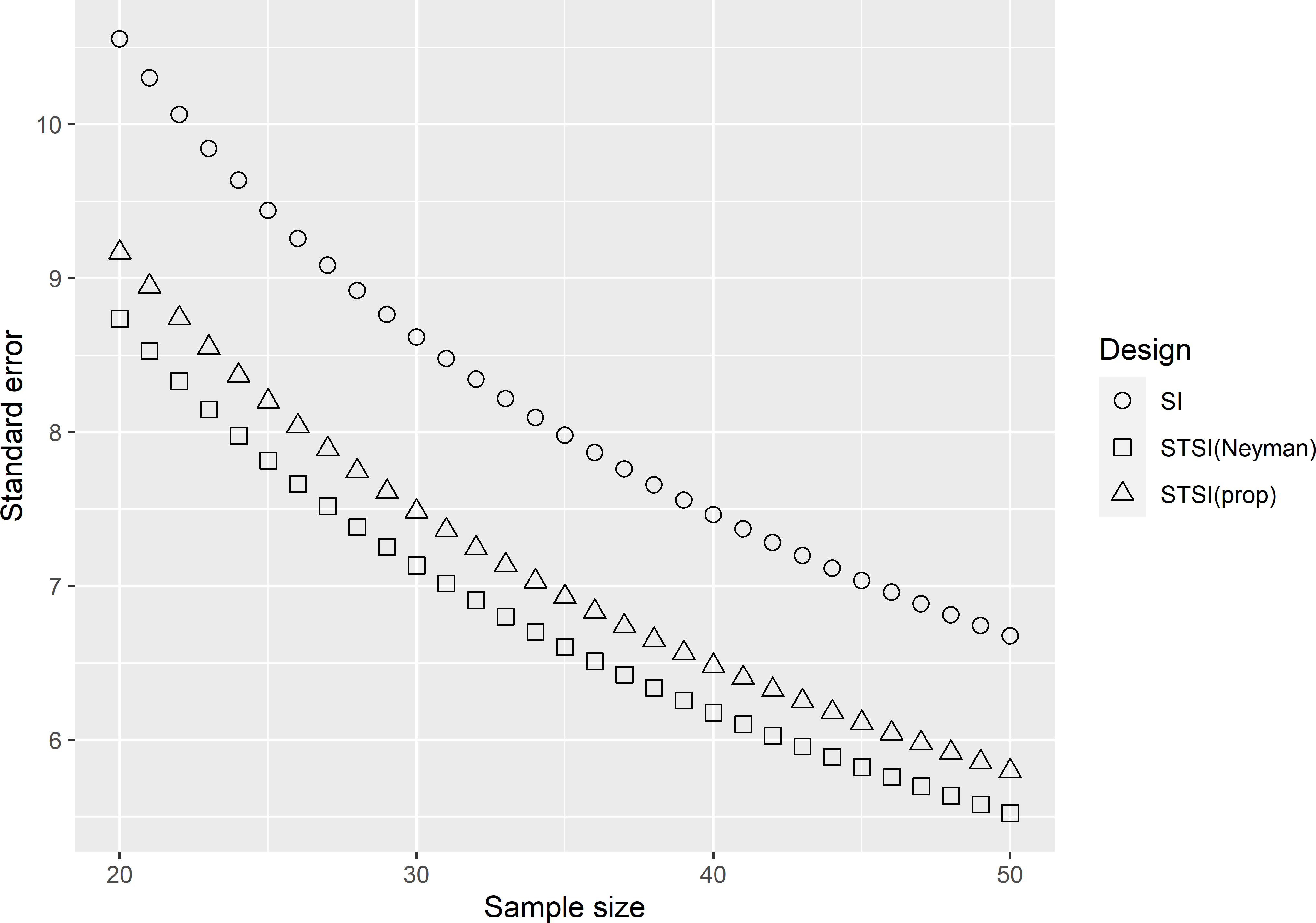
Figure 4.5: Standard error of the \(\pi\) estimator of the mean SOM concentration (g kg-1) as a function of the total sample size, for simple random sampling (SI) and for stratified simple random sampling with proportional (STSI(prop)) and Neyman allocation (STSI(Neyman)) for Voorst.
Optimal allocation and Neyman allocation assume univariate stratification, i.e., the stratified simple random sample is used to estimate the mean of a single study variable. If we have multiple study variables, optimal allocation becomes more complicated. In Bethel allocation, the total sampling costs, assuming a linear costs model (Equation (4.18)), are minimised given a constraint on the precision of the estimated mean for each study variable (Bethel 1989), see Section 4.8. Bethel allocation can be computed with function bethel of package SamplingStrata (G. Barcaroli et al. 2020).
Exercises
- Use function
strataof package sampling to select a stratified simple random sample with replacement of size 40 from Voorst, using proportional allocation. Check that the sum of the stratum sample sizes is 40.- Estimate the population mean and the standard error of the estimator.
- Compute the true standard error of the estimator. Hint: compute the population variances of the study variable \(z\) per stratum, and divide these by the stratum sample sizes.
- Compute a 95% confidence interval estimate of the population mean, using function
confintof package survey.
- Looking at Figure 4.4, which strata do you expect can be merged without losing much precision of the estimated population mean?
- Use function
fct_collapseof package forcats (Hadley Wickham 2021) to merge the strata EA and PA.- Compute the true sampling variance of the estimator of the mean for this new stratification, for a total sample size of 40 and proportional allocation.
- Compare this true sampling variance with the true sampling variance using the original five strata (same sample size, proportional allocation). What is your conclusion about the new stratification?
- Proof that the sum of the inclusion probabilities over all population units with stratified simple random sampling equals the sample size \(n\).
4.4 Cum-root-f stratification
When we have a quantitative covariate \(x\) related to the study variable \(z\) and \(x\) is known for all units in the population, strata can be constructed with the cum-root-f method using this covariate as a stratification variable, see Dalenius and Hodges (1959) and Cochran (1977). Population units with similar values for the covariate (stratification variable) are grouped into a stratum. Strata are computed as follows:
- Compute a frequency histogram of the stratification variable using a large number of bins.
- Compute the square root of the frequencies.
- Cumulate the square root of the frequencies, i.e., compute \(\sqrt{f_1}\), \(\sqrt{f_1} + \sqrt{f_2}\), \(\sqrt{f_1} + \sqrt{f_2} + \sqrt{f_3}\), etc.
- Divide the cumulative sum of the last bin by the number of strata, multiply this value by \(1,2, \dots, H-1\), with H the number of strata, and select the boundaries of the histogram bins closest to these values.
In cum-root-f stratification, it is assumed that the covariate values are nearly perfect predictions of the study variable, so that the prediction errors do not affect the stratification. Under this assumption the stratification is optimal with Neyman allocation of sampling units to the strata 4.3.
Cum-root-f stratification is illustrated with the data of Xuancheng in China. We wish to estimate the mean organic matter concentration in the topsoil (SOM, g kg-1) of this area. Various covariates are available that are correlated with SOM, such as elevation, yearly average temperature, slope, and various other terrain attributes. Elevation, the name of this variable in the tibble is dem, is used as as a single stratification variable, see Figure 4.6. The correlation coefficient of SOM and elevation in a sample of 183 observations is 0.59. The positive correlation can be explained as follows. Temperature is decreasing with elevation, leading to a smaller decomposition rate of organic matter in the soil.
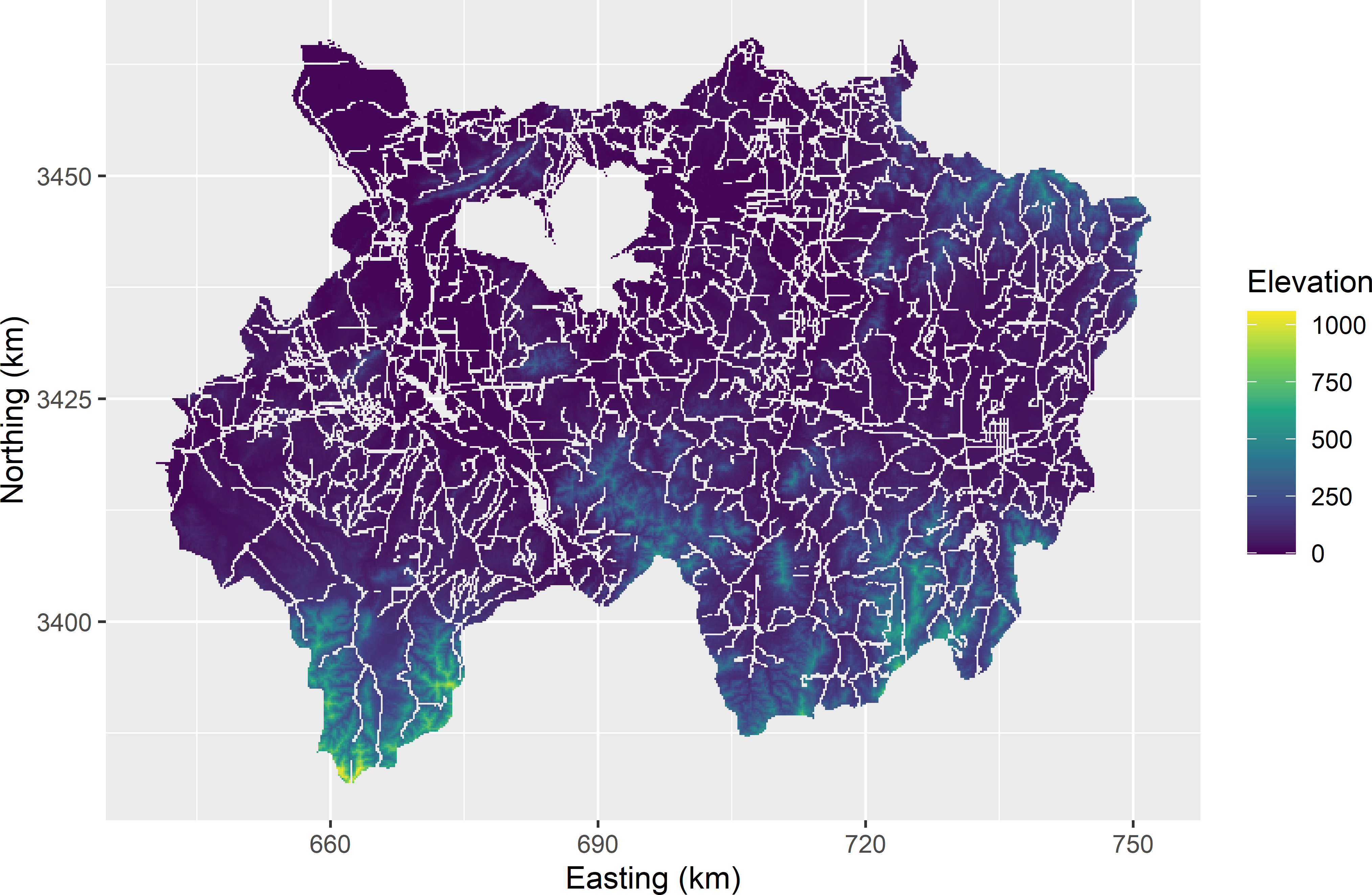
Figure 4.6: Elevation used as a stratification variable in cum-root-f stratification of Xuancheng.
The strata can be constructed with the package stratification (Baillargeon and Rivest 2011). Argument n of this function is the total sample size, but this value has no effect on the stratification. Argument Ls is the number of strata. I arbitrarily chose to construct five strata. Argument nclass is the number of bins of the histogram. The output object of function strata.cumrootf is a list containing amongst others a numeric vector with the stratum bounds (bh) and a factor with the stratum levels of the grid cells (stratumID). Finally, note that the values of the stratification variable must be positive. The minimum elevation is -5 m, so I added the absolute value of this minimum to elevation.
library(stratification)
grdXuancheng <- grdXuancheng %>%
  mutate(dem_new = dem + abs(min(dem)))
crfstrata <- strata.cumrootf(
  x = grdXuancheng$dem_new, n = 100, Ls = 5, nclass = 500)
bh <- crfstrata$bh
grdXuancheng$crfstrata <- crfstrata$stratumID
Stratum bounds are threshold values of the stratification variable elevation; these stratum bounds are equal to 46.7, 108.3, 214.5, 384.4. Note that the number of stratum bounds is one less than the number of strata. The resulting stratification is shown in Figure 4.7. Note that most strata are not single polygons, but are made up of many smaller polygons. This may be even more so if the stratification variable shows a noisy spatial pattern. This is not a problem at all, as a stratum is just a collection of population units (raster cells) and need not be spatially contiguous.
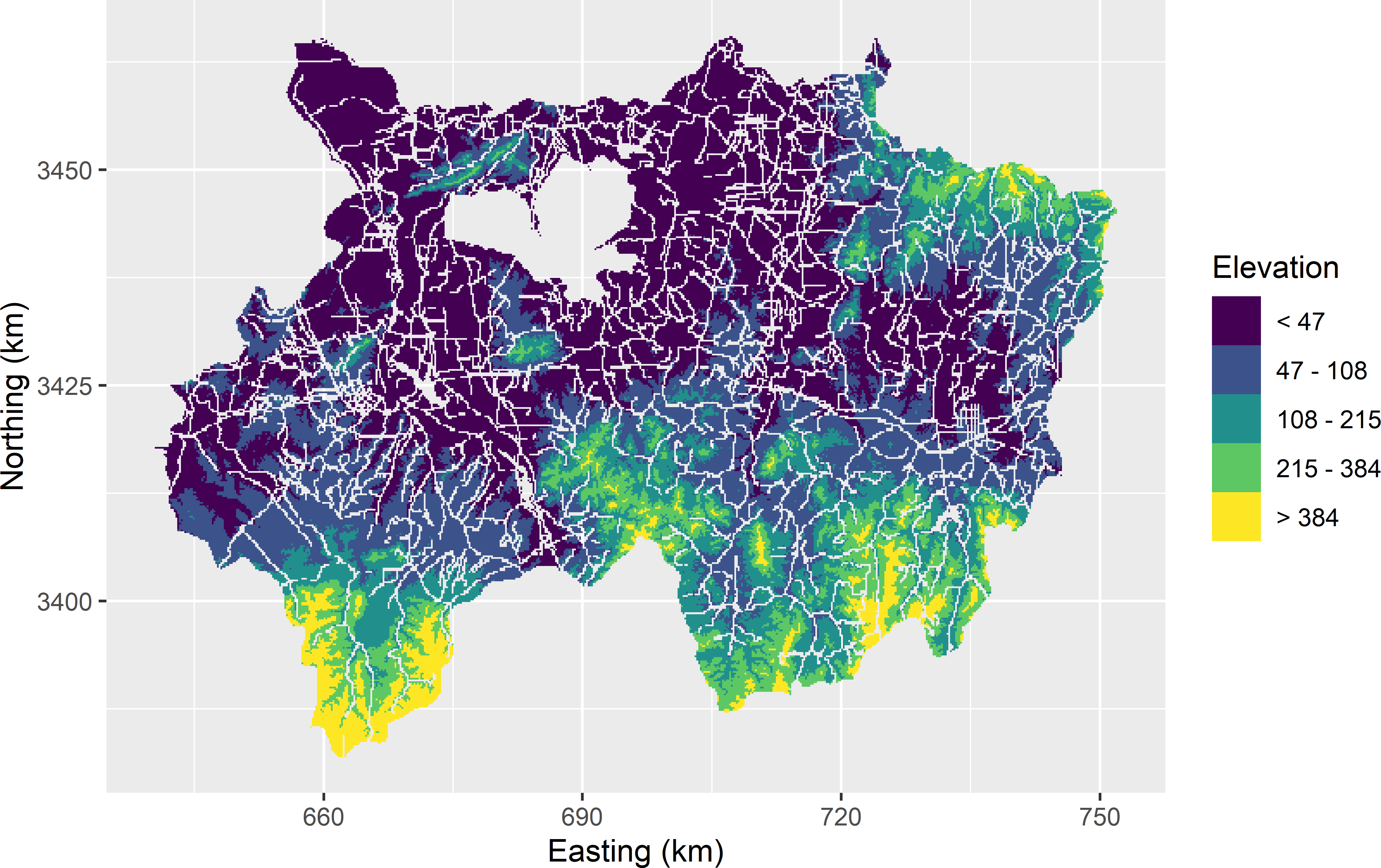
Figure 4.7: Stratification of Xuancheng obtained with the cum-root-f method, using elevation as a stratification variable.
Exercises
- Write an R script to compute five cum-root-f strata for Eastern Amazonia (
grdAmazoniain package sswr) to estimate the population mean of aboveground biomass (AGB), using log-transformed short-wave infrared radiation (SWIR2) as a stratification variable.- Compute ten cum-root-f strata, using function
strataof package sampling. - Select a stratified simple random sample of 100 units. First, compute the stratum sample sizes for proportional allocation.
- Estimate the population mean of AGB and its sampling variance.
- Compute the true sampling variance of the estimator of the mean for this sampling design (see Exercise 1 for a hint).
- Compute the stratification effect (gain in precision). Hint: compute the sampling variance for simple random sampling by computing the population variance of AGB, and divide this by the total sample size.
- Compute ten cum-root-f strata, using function
4.5 Stratification with multiple covariates
If we have multiple variables that are possibly related to the study variable, we may want to use them all or a subset of them as stratification variables. Using the quantitative variables one-by-one in cum-root-f stratification, followed by overlaying the maps with univariate strata, may lead to numerous cross-classification strata.
A simple solution is to construct homogeneous groups, referred to as clusters, of population units (raster cells). The units within a cluster are more similar to each other than to the units in other clusters. Various clustering techniques are available. Here, I use hard k-means.
This is illustrated again with the Xuancheng case study. Five quantitative covariates are used for constructing the strata. Besides elevation, which was used as a single stratification variable in the previous section, now also temperature, slope, topographic wetness index (twi), and profile curvature are used to construct clusters that are used as strata in stratified simple random sampling. To speed up the computations, a subgrid with a spacing of 0.4 km is selected, using function spsample of package sp, see Chapter 5 (Bivand, Pebesma, and Gómez-Rubio 2013).
library(sp)
gridded(grdXuancheng) <- ~ s1 + s2
subgrd <- spsample(
  grdXuancheng, type = "regular", cellsize = 400, offset = c(0.5, 0.5))
subgrd <- data.frame(coordinates(subgrd), over(subgrd, grdXuancheng))
Five clusters are computed with k-means using as clustering variables the five covariates mentioned above. The scale of these covariates is largely different, and for this reason they must be scaled before being used in clustering. The k-means algorithm is a deterministic algorithm, i.e., the same initial clustering will end in the same final, optimised clustering. This final clustering can be suboptimal, and therefore it is recommended to repeat the clustering as many times as feasible, with different initial clusterings. Argument nstart is the number of initial clusterings. The best clustering, i.e., the one with the smallest within-cluster sum-of-squares, is kept.
x <- c("dem", "temperature", "slope", "profile.curvature", "twi")
set.seed(314)
myClusters <- kmeans(
  scale(subgrd[, x]), centers = 5, iter.max = 1000, nstart = 100)
subgrd$cluster <- myClusters$cluster
Figure 4.8 shows the five clusters obtained by k-means clustering of the raster cells. These clusters can be used as strata in random sampling.
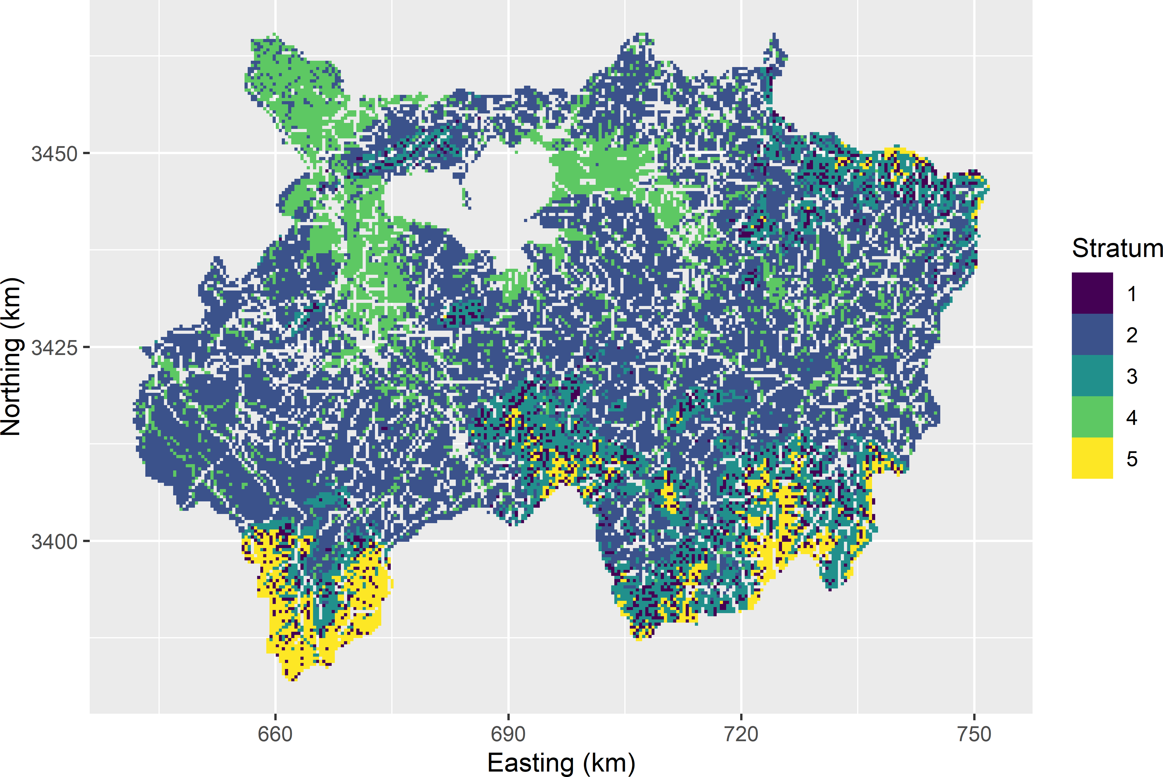
Figure 4.8: Five clusters obtained by k-means clustering of the raster cells of Xuancheng, using five scaled covariates in clustering.
The size of the clusters used as strata is largely different (Table 4.3). This table also shows means of the unscaled covariates used in clustering.
| Stratum | Nh | Elevation | Temperature | Slope | Profilecurv | Twi |
|---|---|---|---|---|---|---|
| 1 | 1,581 | 300 | 14.45 | 12.21 | -0.00147 | 6.34 |
| 2 | 15,987 | 54 | 15.44 | 2.11 | 0.00001 | 9.24 |
| 3 | 4,255 | 181 | 14.64 | 11.11 | 0.00068 | 7.75 |
| 4 | 4,955 | 20 | 15.59 | 0.47 | 0.00006 | 17.08 |
| 5 | 1,625 | 416 | 13.70 | 21.21 | 0.00012 | 6.45 |
Categorical variables can be accommodated in clustering using the technique proposed by Huang (1998), implemented in package clustMixType (Szepannek 2018).
In the situation that we already have some data of the study variable, an alternative solution is to calibrate a model for the study variable, for instance a multiple linear regression model, using the covariates as predictors, and to use the predictions of the study variable as a single stratification variable in cum-root-f stratification or in optimal spatial stratification, see Section 13.2.
4.6 Geographical stratification
When no covariate is available, we may still decide to apply a geographical stratification. For instance, a square study area can be divided into 4 \(\times\) 4 equal-sized subsquares that are used as strata. When we select one or two points per subsquare, we avoid strong spatial clustering of the sampling points. Geographical stratification improves the spatial coverage. When the study variable is spatially structured, think for instance of a spatial trend, then geographical stratification will lead to more precisely estimated means (smaller sampling variances).
A simple method for constructing geographical strata is k-means clustering (Brus, Spätjens, and de Gruijter 1999). See Section 17.2 for a simple illustrative example of how geographical strata are computed with k-means clustering. In this approach, the study area is discretised by a large number of grid cells. These grid cells are the objects that are clustered. The clustering variables are simply the spatial coordinates of the centres of the grid cells. This method leads to compact geographical strata, briefly referred to as geostrata. Geostrata can be computed with function kmeans, as shown in Section 4.5. The two clustering variables have the same scale, so they should not be scaled because this would lead to an arbitrary distortion of geographical distances. The geostrata generally will not have the same number of grid cells. Geostrata of equal size can be attractive, as then the sample becomes selfweighting, i.e., the sample mean is an unbiased estimator of the population mean.
Geostrata of the same size can be computed with function stratify of the package spcosa (D. Walvoort, Brus, and de Gruijter (2020), D. J. J. Walvoort, Brus, and Gruijter (2010)), with argument equalArea = TRUE.
If the total number of grid cells divided by the number of strata is an integer, the stratum sizes are exactly equal; otherwise, the difference is one grid cell. D. J. J. Walvoort, Brus, and Gruijter (2010) describe the k-means algorithms implemented in this package in detail. Argument object of function stratify specifies a spatial object of the population units. In the R code below the subgrid of grdXuancheng generated in Section 4.5 is converted to a SpatialPixelsDataFrame with function gridded of the package sp. The spatial object can also be of class SpatialPolygons. In that case, either argument nGridCells or argument cellSize must be set, so that the vector map in object can be discretised by a finite number of grid cells. Argument nTry specifies the number of initial stratifications in k-means clustering, and therefore is comparable with argument nstart of function kmeans. For more details on spatial stratification using k-means clustering, see Section 17.2. The k-means algorithm used with equalArea = TRUE takes much more computing time than the one used with equalArea = FALSE.
library(spcosa)
library(sp)
set.seed(314)
gridded(subgrd) <- ~ x1 + x2
mygeostrata <- stratify(
  object = subgrd, nStrata = 50, nTry = 1, equalArea = TRUE)
Function spsample of package spcosa is used to select from each geostratum a simple random sample of two points.
Figure 4.9 shows fifty compact geostrata of equal size for Xuancheng with the selected sampling points. Note that the sampling points are reasonably well spread throughout the study area2.
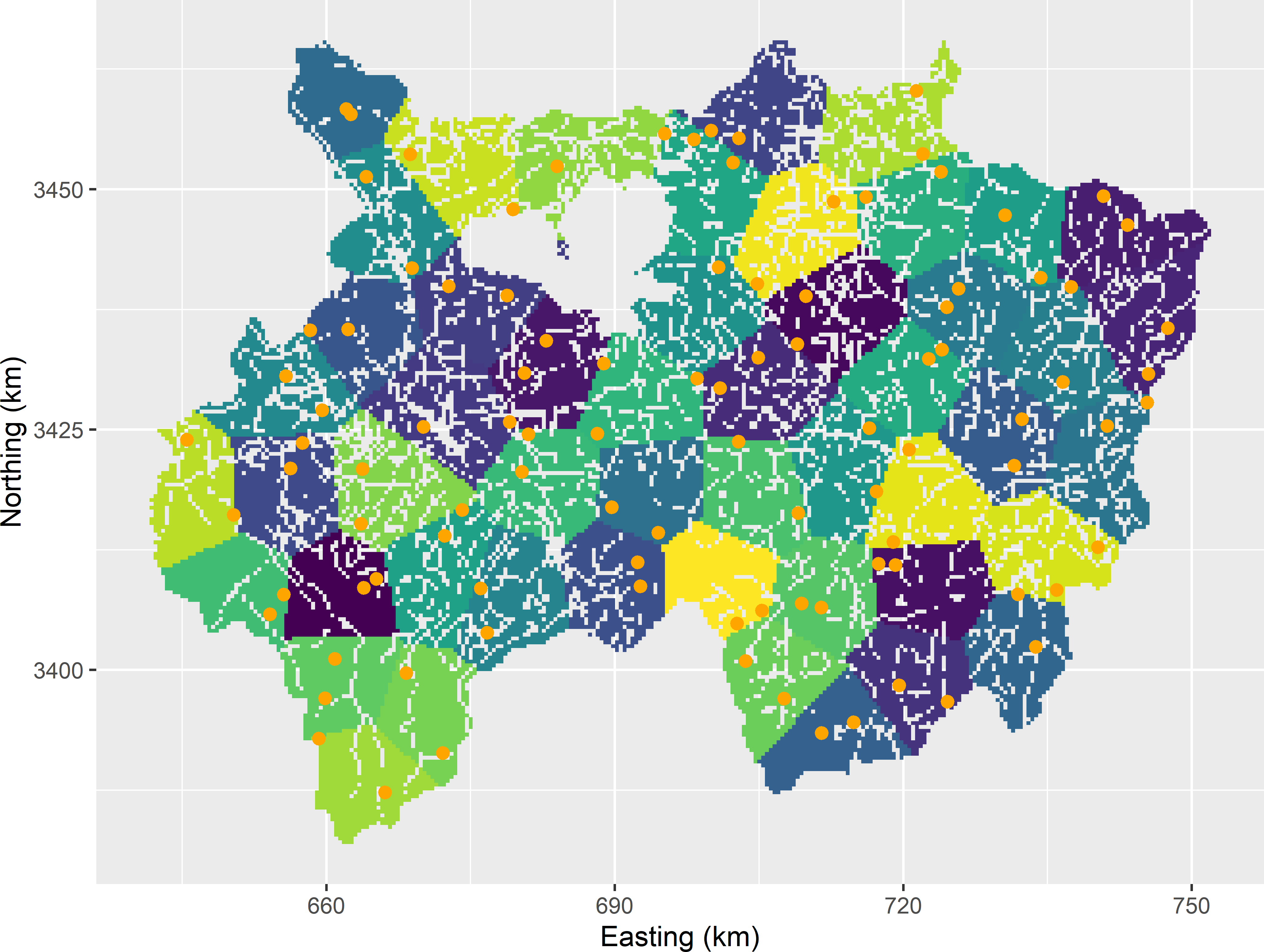
Figure 4.9: Compact geostrata of equal size for Xuancheng and stratified simple random sample of two points per stratum.
Once the observations are done, the population mean can be estimated with function estimate. For Xuancheng I simulated data from a normal distribution, just to illustrate estimation with function estimate. Various statistics can be estimated, among which the population mean (spatial mean), the standard error, and the CDF. The CDF is estimated by transforming the data into indicators (Subsection 3.1.2).
library(spcosa)
mysample <- spcosa::spsample(mygeostrata, n = 2)
mydata <- data.frame(z = rnorm(100, mean = 10, sd = 2))
mean <- estimate("spatial mean", mygeostrata, mysample, data = mydata)
se <- estimate("standard error", mygeostrata, mysample, data = mydata)
cdf <- estimate("scdf", mygeostrata, mysample, data = mydata)
The estimated population mean equals 9.8 with an estimated standard error of 0.2.
Exercises
- Why is it attractive to select at least two points per geostratum?
- The alternative to 50 geostrata and two points per geostratum is 100 geostrata and one point per geostratum. Which sampling strategy will be more precise?
- The geostrata in Figure 4.9 have equal size (area), which can be enforced by argument
equalArea = TRUE. Why are equal sizes attractive? Work out the estimator of the population mean for strata of equal size.
- Write an R script to construct 20 compact geographical strata of equal size for agricultural field Leest. The geopackage file of this field can be read with sf function
read_sf(system.file("extdata/leest.gpkg", package = "sswr")). Remove the projection attributes withst_set_crs(NA_crs_), and convert the simple feature object to a spatial object with methodas_Spatial. Select two points per geostratum, using functionspsampleof package spcosa. Repeat this with 40 strata of equal size, and randomly select one point per stratum.- If only one point per stratum is selected, the sampling variance can be approximated by the collapsed strata estimator. In this method, pairs of strata are formed, and the two strata of a pair are joined. In each new stratum we now have two points. With an odd number of strata there will be one group of three strata and three points. The sample is then analysed as if it were a random sample from the new collapsed strata. Suppose we group the strata on the basis of the measurements of the study variable. Do you think this is a proper way of grouping?
- In case you think this is not a proper way of grouping the strata, how would you group the strata?
- Is the sampling variance estimator unbiased? If not, is the sampling variance overestimated or underestimated?
- Laboratory costs for measuring the study variable can be saved by bulking the soil aliquots (composite sampling). There are two options: bulking all soil aliquots from the same stratum (bulking within strata) or bulking by selecting one aliquot from each stratum (bulking across strata). In spcosa bulking across strata is implemented. Write an R script to construct 20 compact geographical strata for study area Voorst. Use argument
equalArea = TRUE. Select four points per stratum using argumenttype = "composite", and convert the resulting object toSpatialPoints. Extract the \(z\)-values ingrdVoorstat the selected sampling points using functionover. Add a variable to the resulting data frame indicating the composite (points 1 to 4 are from the first stratum, points 5 to 8 from the second stratum, etc.), and estimate the means for the four composites using functiontapply. Finally, estimate the population mean and its standard error.- Can the sampling variance of the estimator of the mean be estimated for bulking within the strata?
- The alternative to analysing the concentration of four composite samples obtained by bulking across strata is to analyse all 20 \(\times\) 4 aliquots separately. The strata have equal size, so the inclusion probabilities are equal. As a consequence, the sample mean is an unbiased estimator of the population mean. Is the precision of this estimated population mean equal to that of the estimated population mean with composite sampling? If not, is it smaller or larger, and why?
- If you use argument
equalArea = FALSEin combination with argumenttype = "composite", you get an error message. Why does this combination of arguments not work?
4.7 Multiway stratification
In Section 4.5 multiple continuous covariates are used to construct clusters of raster cells using k-means. These clusters are then used as strata. This section considers the case where we have multiple categorical and/or continuous variables that we would like to use as stratification variables. The continuous stratification variables are first used to compute strata based on that stratification variable, e.g., using the cum-root-f method. What could be done then is to compute the cross-classification of each unit and use these cross-classifications as strata in random sampling. However, this may lead to numerous strata, maybe even more than the intended sample size. To reduce the total number of strata, we may aggregate cross-classification strata with similar means of the study variable, based on our prior knowledge.
An alternative to aggregation of cross-classification strata is to use the separate strata, i.e., the strata based on an individual stratification variable, as marginal strata in random sampling. How this works is explained in Subsection 9.1.4.
4.8 Multivariate stratification
Another situation is where we have multiple study variables and would like to optimise the stratification and allocation for estimating the population means of all study variables. Optimal stratification for multiple study variables is only relevant if we would like to use different stratification variables for the study variables. In many cases, we do not have reliable prior information about the different study variables justifying the use of multiple stratification variables. We are already happy to have one stratification variable that may serve to increase the precision of the estimated means of all study variables.
However, in case we do have multiple stratification variables tailored to different study variables, the objective is to partition the population in strata, so that for a given allocation, the total sampling costs, assuming a linear costs model (Equation (4.18)), are minimised given a constraint on the precision of the estimated mean for each study variable.
Package SamplingStrata (G. Barcaroli et al. 2020) can be used to optimise multivariate strata. Giulio Barcaroli (2014) gives details about the objective function and the algorithm used for optimising the strata. Sampling units are allocated to the strata by Bethel allocation (Bethel 1989). The required precision is specified in terms of a coefficient of variation, one per study variable.
Multivariate stratification is illustrated with the Meuse data set of package gstat (E. J. Pebesma 2004). The prior data of heavy metal concentrations of Cd and Zn are used in spatial prediction to create maps of these two study variables.
The maps of natural logs of the two metal concentrations are created by kriging with an external drift, using the square root of the distance to the Meuse river as a predictor for the mean, see Section 21.3 for how this spatial prediction method works.
Figure 4.10 shows the map with the predicted log Cd and log Zn concentrations.
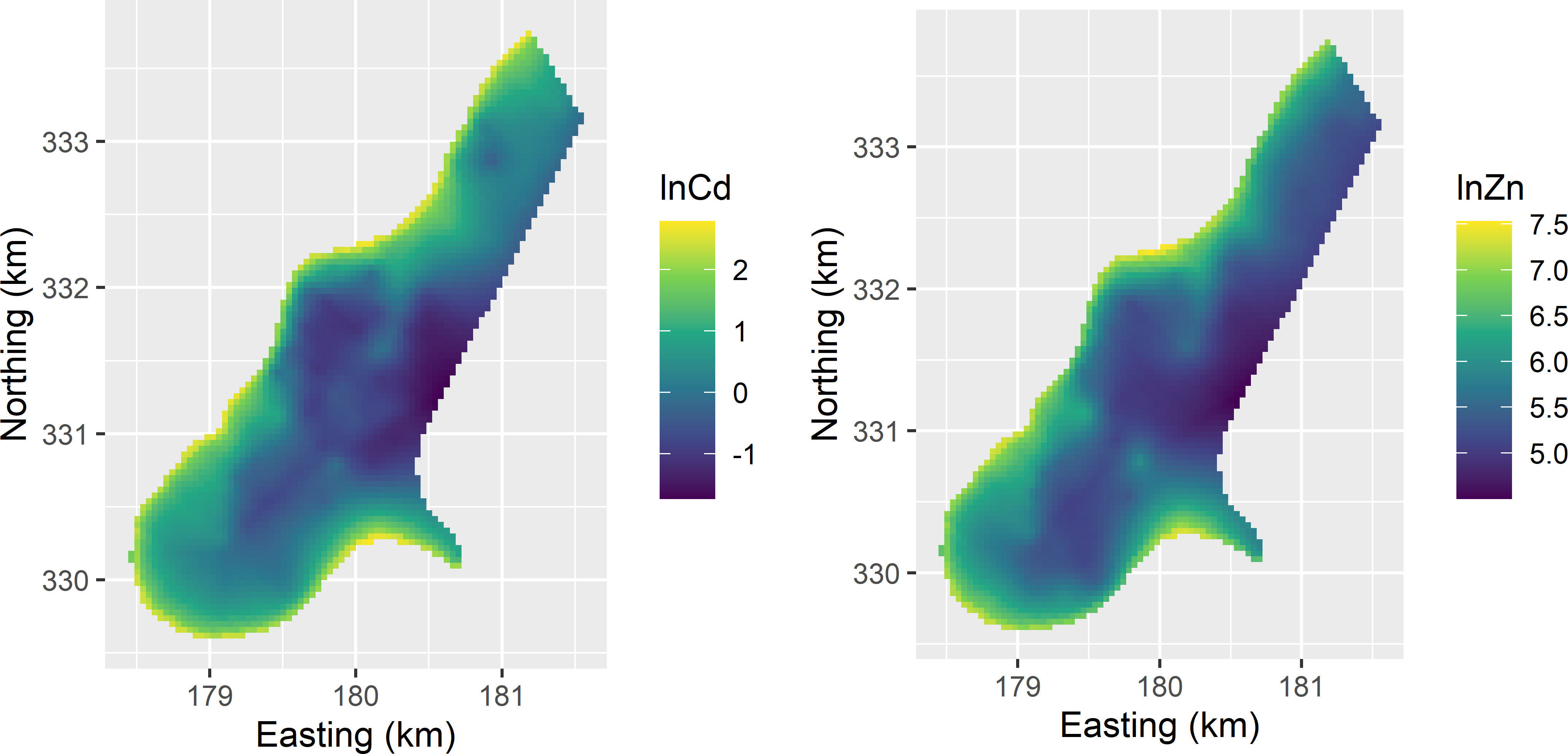
Figure 4.10: Kriging predictions of natural logs of Cd and Zn concentrations in the study area Meuse, used as stratification variables in bivariate stratification.
The predicted log concentrations of the two heavy metals are used as stratification variables in designing a new sample for design-based estimation of the population means of Cd and Zn. For the log of Cd, there are negative predicted concentrations (Figure 4.10). This leads to an error when running function optimStrata. The minimum predicted log Cd concentration is -1.7, so I added 2 to the predictions. A variable indicating the domains of interest is added to the data frame. The value of this variable is 1 for all grid cells, so that a sample is designed for estimating the mean of the entire population. As a first step, function buildFrameDF is used to create a data frame that can be handled by function optimStrata. Argument X specifies the stratification variables, and argument Y the study variables. In our case, the stratification variables and the study variables are the same. This is typical for the situation where the stratification variables are obtained by mapping the study variables.
library(SamplingStrata)
df <- data.frame(cd = lcd_kriged$var1.pred + 2,
                 zn = lzn_kriged$var1.pred,
                 dom = 1,
                 id = seq_len(nrow(lcd_kriged)))
frame <- buildFrameDF(
  df = df, id = "id",
  X = c("cd", "zn"), Y = c("cd", "zn"),
  domainvalue = "dom")
Next, a data frame with the precision requirements for the estimated means is created. The precision requirement is given as a coefficient of variation, i.e., the standard error of the estimated population mean, divided by the estimated mean. The study variables as specified in Y are used to compute the estimated means and the standard errors for a given stratification and allocation.
Finally, the multivariate stratification is optimised by searching for the optimal stratum bounds using a genetic algorithm (Gershenfeld 1999).
set.seed(314)
res <- optimStrata(
  method = "continuous",  errors = cv, framesamp = frame, nStrata = 5,
  iter = 50, pops = 20, showPlot = FALSE)
A summary of the strata can be obtained with function summaryStrata.
  Stratum Population Allocation Lower_X1 Upper_X1 Lower_X2 Upper_X2
1       1        717          7    0.266    1.421    4.502    5.576
2       2        694          5    1.421    2.090    4.950    6.010
3       3        597          3    2.091    2.630    5.163    6.358
4       4        704          6    2.630    3.476    5.472    6.802
5       5        391          5    3.480    4.781    6.234    7.527
Column Population contains the sizes of the strata, i.e., the number of grid cells. The total sample size equals 26. The sample size per stratum is computed with Bethel allocation, see Section 4.3. The last four columns contain the lower and upper bounds of the orthogonal intervals.
Figure 4.11 shows a 2D-plot of the bivariate strata. The strata can be plotted as a series of nested rectangles. All population units in the smallest rectangle belong to stratum 1; all units in the one-but-smallest rectangle that are not in the smallest rectangle belong to stratum 2, etc. If we have more than two stratification variables, the strata form a series of nested hyperrectangles or boxes. The strata are obtained as the Cartesian product of orthogonal intervals.
plt <- plotStrata2d(res$framenew, res$aggr_strata,
  domain = 1, vars = c("X1", "X2"), labels = c("Cd", "Zn"))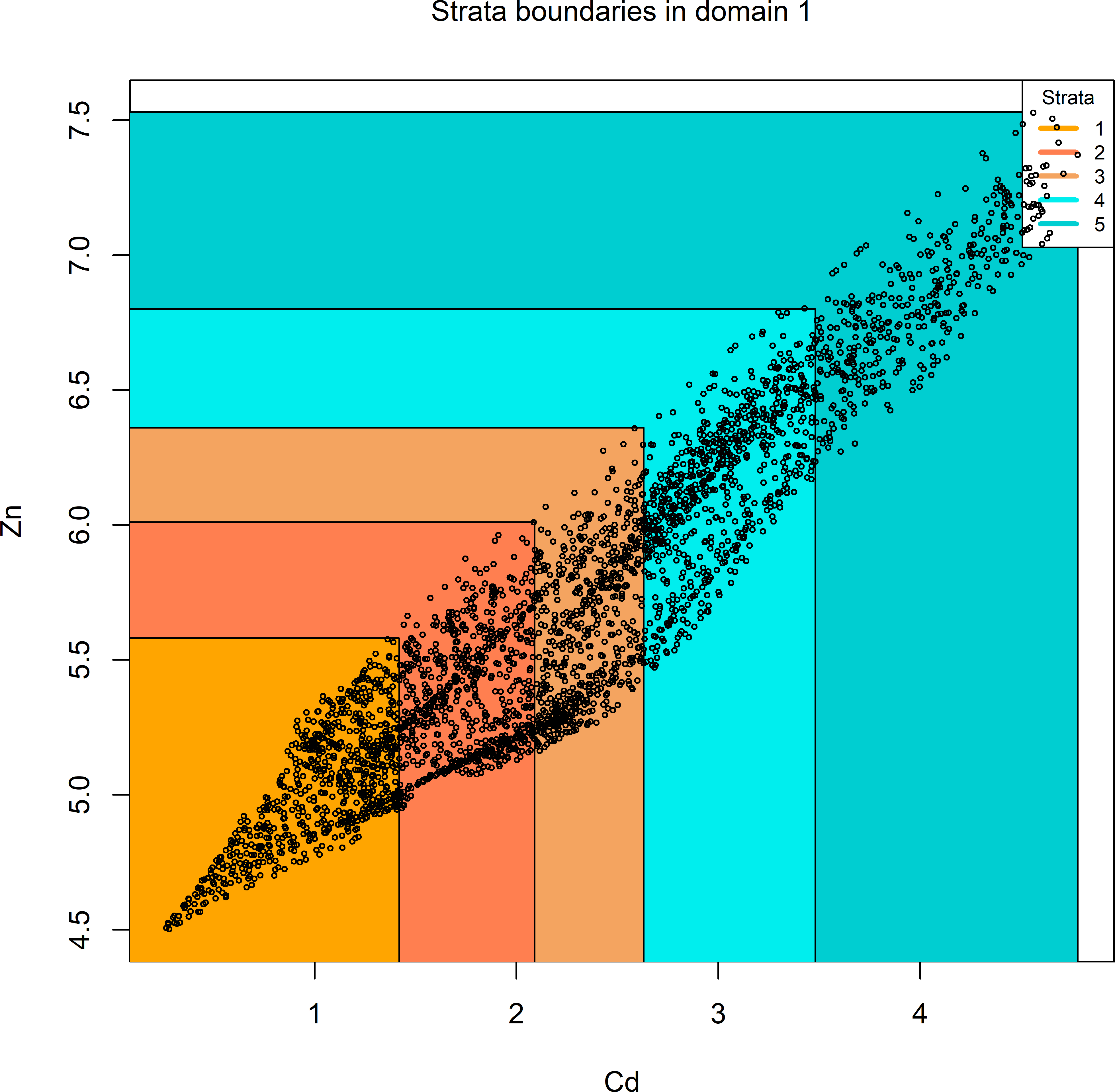
Figure 4.11: 2D-plot of optimised bivariate strata of the study area Meuse.
Figure 4.12 shows a map of the optimised strata.
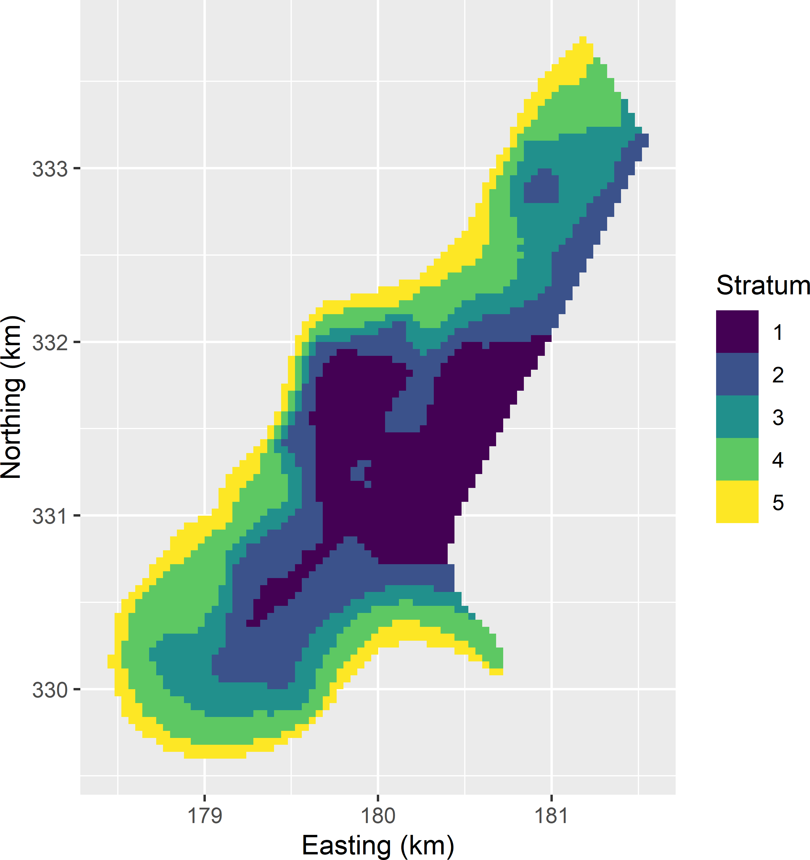
Figure 4.12: Map of optimised bivariate strata of the study area Meuse.
The expected coefficient of variation can be extracted with function expected_CV.
     cv(Y1)    cv(Y2)
DOM1   0.02 0.0087401
The coefficient of variation of Cd is indeed equal to the desired level of 0.02, for Zn it is smaller. So, in this case Cd is the study variable that determines the total sample size of 26 units.
Note that these coefficients of variation are computed from the stratification variables, which are predictions of the study variable. Errors in these predictions are not accounted for. It is well known that kriging is a smoother, so that the variance of the predicted values within a stratum is smaller than the variance of the true values. As a consequence, the coefficients of variation of the predictions underestimate the coefficients of variation of the study variables. See Section 13.2 for how prediction errors and spatial correlation of prediction errors can be accounted for in optimal stratification. An additional problem is that I added a value of 2 to the log Cd concentrations. This does not affect the standard error of the estimated mean, but does affect the estimated mean, so that also for this reason the coefficient of variation of the study variable Cd is underestimated.
References
The compact geostrata and the sample are plotted with package ggplot2. A simple alternative is to use method
plotof spcosa:plot(mygeostrata, mysample).↩︎