Chapter 20 Spatial response surface sampling
As with conditioned Latin hypercube sampling, spatial response surface sampling is an experimental design adapted for spatial surveys. Experimental response surface designs aim at finding an optimum of the response within specified ranges of the factors. There are many types of response surface designs, see Myers, Montgomery, and Anderson-Cook (2009). With response surface sampling one assumes that some type of low order regression model can be used to accurately approximate the relationship between the study variable and the covariates. A commonly used design is the central composite design. The data obtained with this design are used to fit a multiple linear regression model with quadratic terms, yielding a curved, quadratic surface of the response.
The response surface sampling approach is an adaptation of an experimental design, but at the same time it is an example of a model-based sampling design. Sampling units are selected to implicitly optimise the estimation of the quadratic regression model. However, this optimisation is done under one or more spatial constraints. Unconstrained optimisation of the sampling design under the linear regression model will not prevent the units from spatial clustering, see the optimal sample in Figure 16.1. The assumption of independent data might be violated when the sampling units are spatially clustered. For this reason, the response surface sampling design selects samples with good spatial coverage, so that the design becomes robust against violation of the independence assumption.
Lesch, Strauss, and Rhoades (1995) adapted the response surface methodology for observational studies. Several problems needed to be tackled. First, when multiple covariates are used, the covariates must be decorrelated. Second, when sampling units are spatially clustered, the assumption in linear regression modelling of spatially uncorrelated model residuals can be violated. To address these two problems, Lesch, Strauss, and Rhoades (1995) proposed the following procedure; see also Lesch (2005):
- Transform the covariate matrix into a scaled, centred, decorrelated matrix by principal components analysis (PCA).
- Choose the response surface design type.
- Select candidate sampling units based on the distance from the design points in the space spanned by the principal components. Select multiple sampling units per design point.
- Select the combination of candidate sampling units with the highest value for a criterion that quantifies how uniform the sample is spread across the study area.
This design has been applied, among others, for mapping soil salinity (ECe), using electromagnetic (EM) induction measurements and surface array conductivity measurements as predictors in multiple linear regression models. For applications, see Corwin and Lesch (2005), Lesch (2005), Fitzgerald et al. (2006), Corwin et al. (2010), and Fitzgerald (2010).
Spatial response surface sampling is illustrated with the EM measurements (mS m-1) of the apparent electrical conductivity on the 80 ha Cotton Research Farm in Uzbekistan. The EM measurements in vertical dipole mode, with transmitter at 1 m and 0.5 m from the receiver, are on transects covering the Cotton Research Farm (Figure 20.1). As a first step, the natural log of the two EM measurements, denoted by lnEM, are interpolated by ordinary kriging to a fine grid (Figure 20.2). These ordinary kriging predictions of lnEM are used as covariates in response surface sampling. The two covariates are strongly correlated, \(r=0.73\), as expected since they are interpolations of measurements of the same variable but of different overlapping layers.
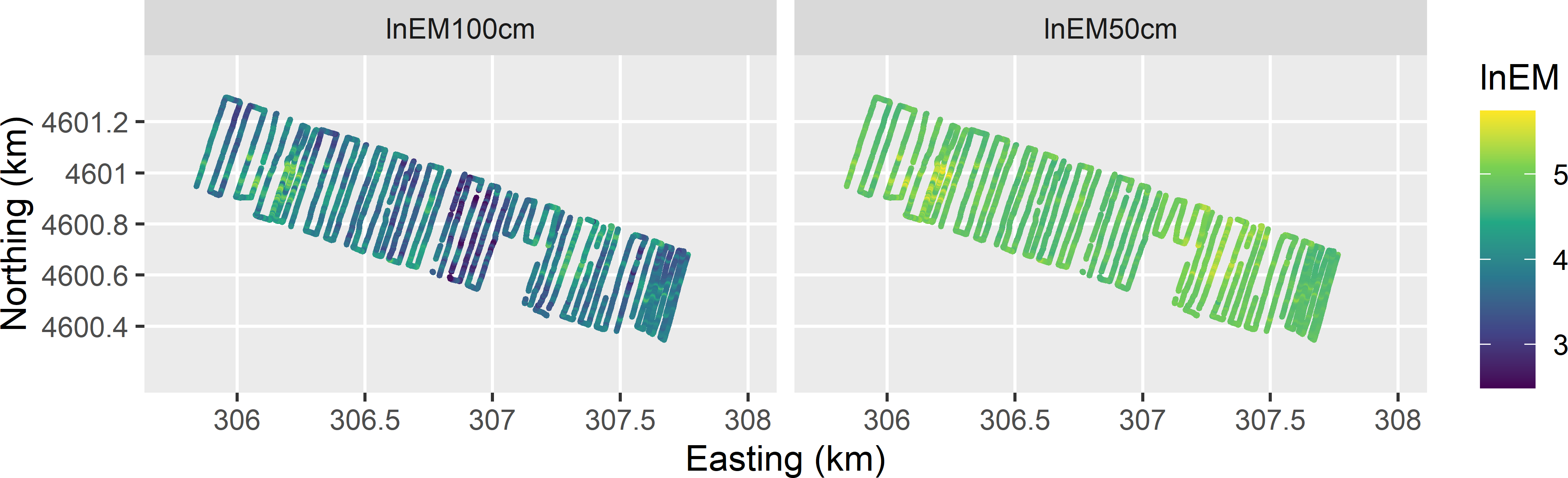
Figure 20.1: Natural log of EM measurements on the Cotton Research Farm (with transmitter at 1 m and 0.5 m from receiver).
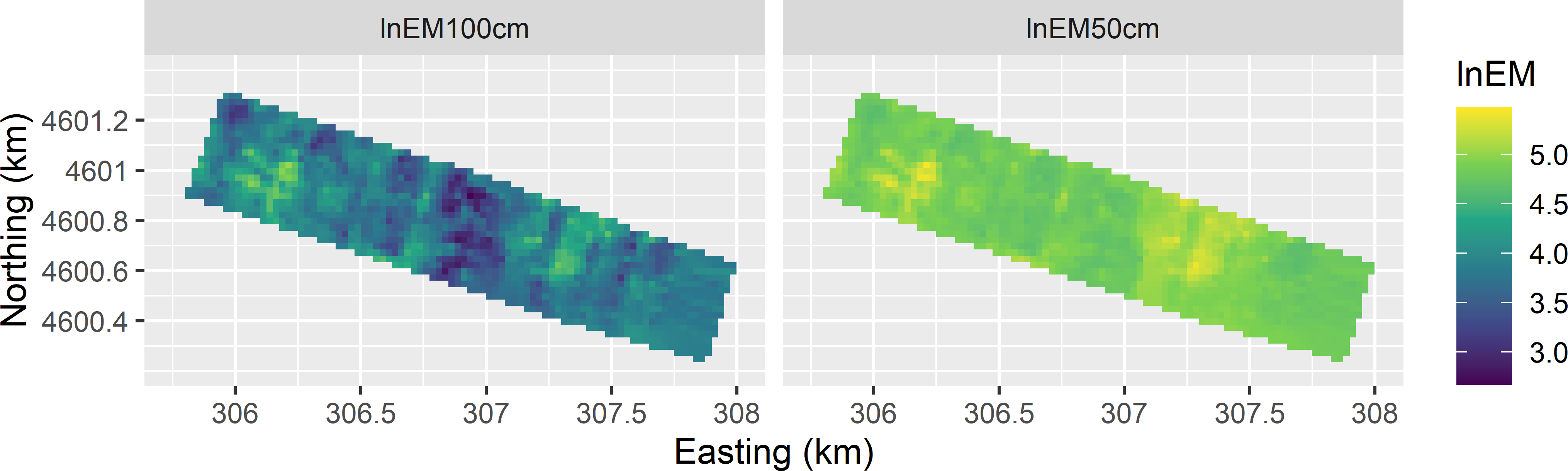
Figure 20.2: Interpolated surfaces of natural log of EM measurements on the Cotton Research Farm, used as covariates in spatial response surface sampling.
Function prcomp of the stats package (R Core Team 2021) is used to compute the principal component scores for all units in the population (grid cells). The two covariates are centred and scaled, i.e., standardised principal components are computed.
The means of the two principal component scores are 0; however, their standard deviations are not zero but 1.330 and 0.480. Therefore, the principal component scores are divided by these standard deviations. They then will have the same weight in the following steps.
Function ccd of package rsm (Lenth 2009) is now used to generate a central composite response surface design (CCRSD). Argument basis specifies the number of factors, which is two in our case. Argument n0 is the number of centre points, and argument alpha determines the position of the star points (explained hereafter).
   run.order std.order  x1.as.is  x2.as.is Block
1          1         4  1.000000  1.000000     1
2          2         5  0.000000  0.000000     1
3          3         2  1.000000 -1.000000     1
4          4         1 -1.000000 -1.000000     1
5          5         3 -1.000000  1.000000     1
6          1         5  0.000000  0.000000     2
7          2         3  0.000000 -1.414214     2
8          3         1 -1.414214  0.000000     2
9          4         4  0.000000  1.414214     2
10         5         2  1.414214  0.000000     2

Data are stored in coded form using these coding formulas ...
x1 ~ x1.as.is
x2 ~ x2.as.is
The experiment consists of two blocks, each of five experimental units. Block 1, the so-called cube block, consists of one centre point and four cube points. In the experimental unit represented by the centre point, both factors have levels in the centre of the experimental range. In the experimental units represented by the cube points, the levels of both factors is either -1 or +1 unit in the design space. Block 2, referred to as the star block, consists of one centre point and four star points. With alpha = "rotatable" the star points are on the circle circumscribing the square (Figure 20.3).
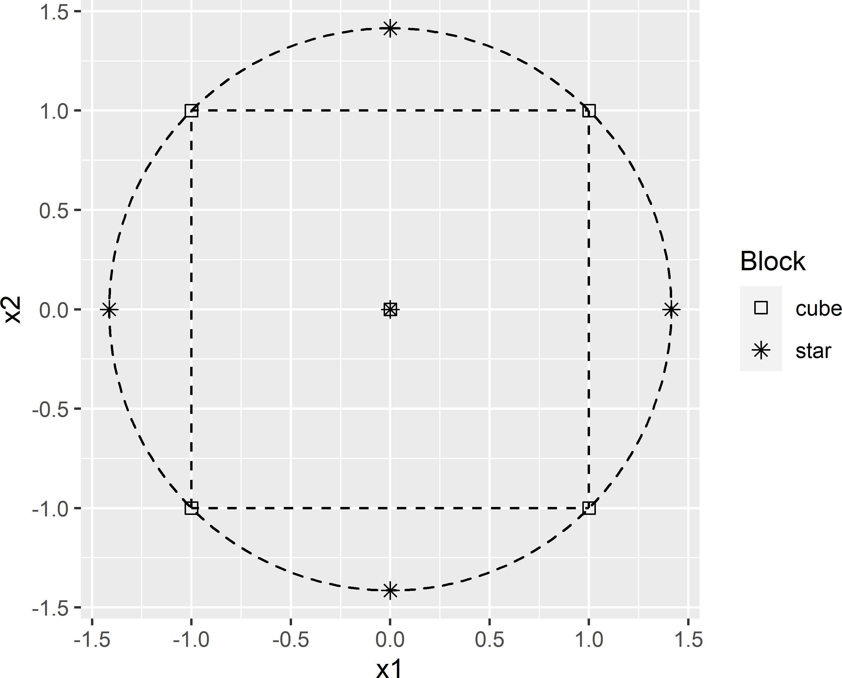
Figure 20.3: Rotatable central composite design for two factors.
To adapt this design for an observational study, we drop one of the centre points (0,0).
The coordinates of the CCRSD points are multiplied by a factor so that a large proportion \(p\) of the bivariate standardised principal component scores of the population units is covered by the circle that passes through the design points (Figure 20.3). The factor is computed as a sample quantile of the empirical distribution of the distances of the points in the scatter to the centre. For \(p\), I chose 0.7.
     70%
1.472547 The next step is to select for each design point several candidate sampling points. For each of the nine design points, eight points are selected that are closest to that design point. This results in 9 \(\times\) 8 candidate sampling points.
candi_all <- NULL
for (i in seq_len(nrow(ccd_df))) {
    d2dpnt <- sqrt((grdCRF$PC1 - ccd_df$x1[i])^2 +
      (grdCRF$PC2 - ccd_df$x2[i])^2)
    grdCRF <- grdCRF[order(d2dpnt), ]
    candi <- grdCRF[c(1:8), c("point_id", "x", "y", "PC1", "PC2")]
    candi$dpnt <- i
    candi_all <- rbind(candi_all, candi)
}
Figure 20.4 shows the nine clusters of candidate sampling points around the design points. Note that the location of the candidate sampling points associated with the design points with coordinates (0,-2.13), (1.51,-1.51), and (2.13,0) are all far inside the circle that passes through the design points. So, for the optimised sample, there will be three points with principal component scores that considerably differ from the ideal values according to the CCRSD design.
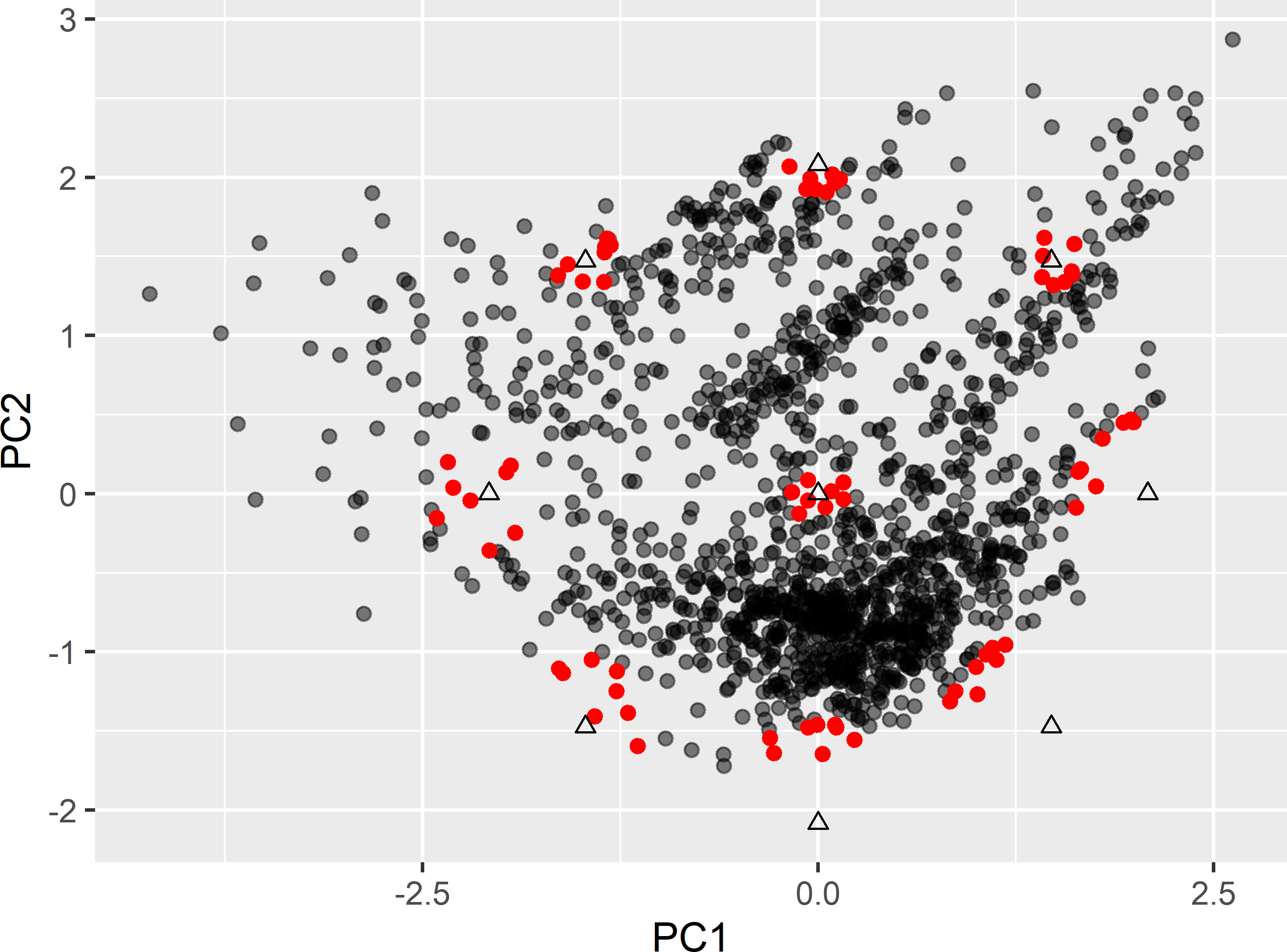
Figure 20.4: Clusters of points (red points) around the design points (triangles) of a CCRSD (two covariates), serving as candidate sampling points.
Figure 20.5 shows that in geographical space for most design points there are multiple spatial clusters of candidate units. For instance, for design point nine, there are three clusters of candidate sampling units. Therefore, there is scope to optimise the sample computationally.
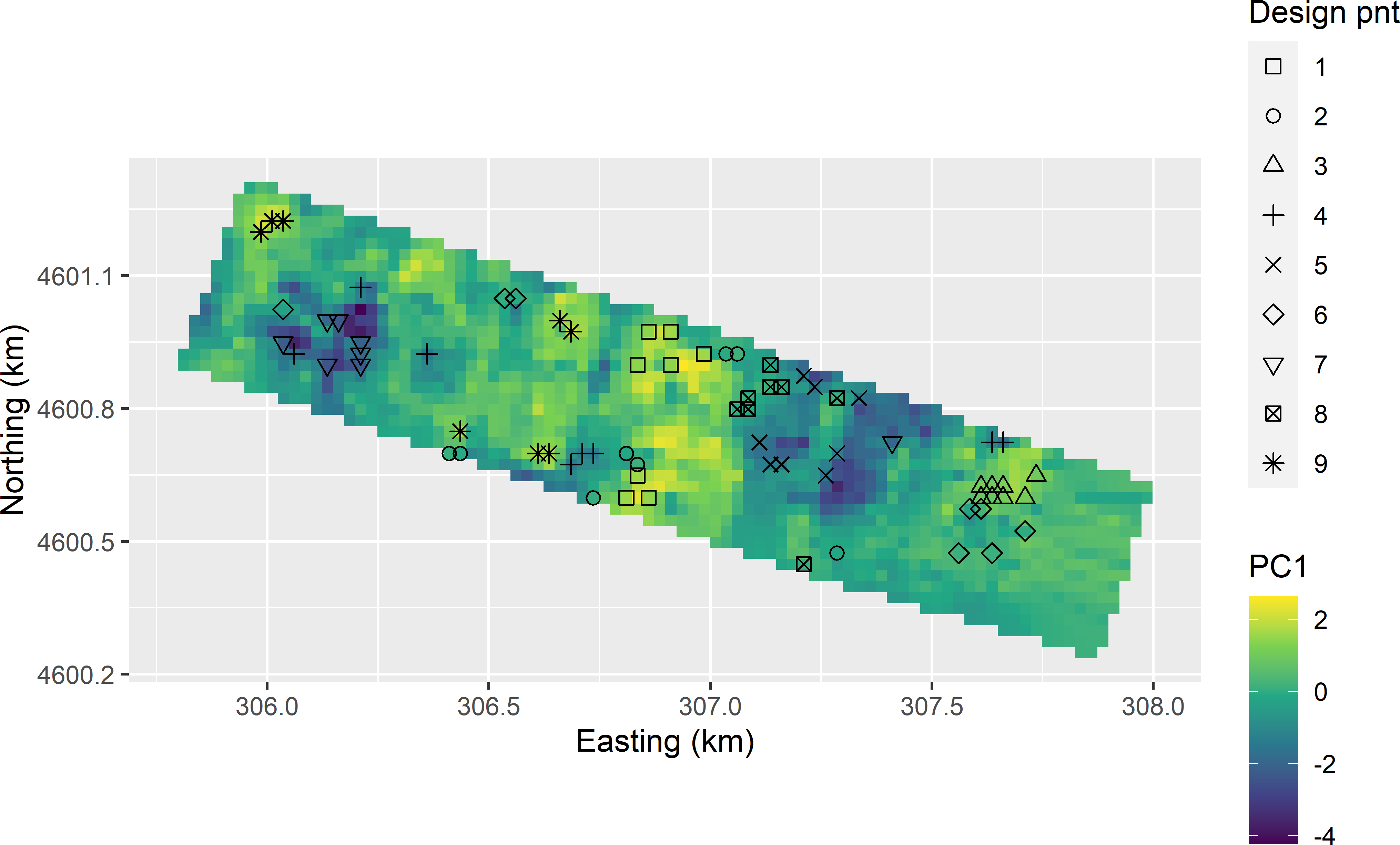
Figure 20.5: Candidate sampling points plotted on a map of the first standardised principal component (PC1).
As a first step, an initial subsample from the candidate sampling units is selected by stratified simple random sampling, using the levels of factor dpnt as strata. Function strata of package sampling is used for stratified random sampling (Tillé and Matei 2021).
library(sampling)
set.seed(314)
units_stsi <- sampling::strata(
  candi_all, stratanames = "dpnt", size = rep(1, 9))
mysample0 <- getdata(candi_all, units_stsi) %>%
  dplyr::select(-(ID_unit:Stratum))
The locations of the nine sampling units are now optimised by minimising a criterion that is a function of the distance between the nine sampling points. Two minimisation criteria are implemented, a geometric criterion and a model-based criterion.
In the geometric criterion (as proposed by Lesch (2005)) for each sampling point the log of the shortest distance to the other points is computed. The minimisation criterion is the negative of the sample mean of these distances.
The model-based minimisation criterion is the average correlation of the sampling points. This criterion requires as input the parameters of a residual correlogram (see Section 21.3). I assume an exponential correlogram without nugget, so that the only parameter to be chosen is the distance parameter \(\phi\) (Equation (21.13)). Three times \(\phi\) is referred to as the effective range of the exponential correlogram. The correlation of the random variables at two points separated by this distance is 0.05.
A penalty term is added to the geometric or the model-based minimisation criterion, equal to the average distance of the sampling points to the associated design points, multiplied by a weight. With weights \(>0\), sampling points close to the design points are preferred over more distant points.
In the next code chunk, a function is defined for computing the minimisation criterion. Given a chosen value for \(\phi\), the 9 \(\times\) 9 distance matrix of the sampling points can be converted into a correlation matrix, using function variogramLine of package gstat (E. J. Pebesma 2004). Argument weight is an optional argument with default value 0.
getCriterion <- function(mysample, dpnt, weight = 0, phi = NULL) {
  D2dpnt <- sqrt((mysample$PC1 - dpnt$x1)^2 + (mysample$PC2 - dpnt$x2)^2)
  D <- as.matrix(dist(mysample[, c("x", "y")]))
  if (is.null(phi)) {
    diag(D) <- NA
    logdmin <- apply(D, MARGIN = 1, FUN = min, na.rm = TRUE) %>% log
    criterion_cur <- mean(-logdmin) + mean(D2dpnt) * weight
  } else {
    vgmodel <- vgm(model = "Exp", psill = 1, range = phi)
    C <- variogramLine(vgmodel, dist_vector = D, covariance = TRUE)
    criterion_cur <- mean(C) + mean(D2dpnt) * weight
  }
  return(criterion_cur)
}
Function getCriterion is used to compute the geometric criterion for the initial sample.
The initial value of the geometric criterion is -4.829. In the next code chunk, the initial value for the model-based criterion is computed for an effective range of 150 m.
The initial value of the model-based criterion is 0.134.
The objective function defining the minimisation criterion is minimised with simulated annealing (Kirkpatrick, Gelatt, and Vecchi (1983), Aarts and Korst (1989)). One sampling point is randomly selected and replaced by another candidate sampling point from the same cluster. If the criterion of the new sample is smaller than that of the current sample, the new sample is accepted. If it is larger, it is accepted with a probability that is a function of the change in the criterion (the larger the increase, the smaller the acceptance probability) and of an annealing parameter named the temperature (the higher the temperature, the larger the probability of accepting a new, poorer sample, given an increase of the criterion). See Section 23.1 for a more detailed introduction to simulated annealing.
The sampling pattern can be optimised with function anneal of package sswr. The arguments of this function will be clear from the description of the sampling procedure above.
set.seed(314)
mySRSsample <- anneal(
  mysample = mysample0, candidates = candi_all, dpnt = ccd_df, phi = 50,
  T_ini = 1, coolingRate = 0.9, maxPermuted = 25 * nrow(mysample0),
  maxNoChange = 20, verbose = TRUE)
Figure 20.6 shows the optimised CCRSD samples plotted in the space spanned by the two principal components, obtained with the geometric and the model-based criterion, plotted together with the design points. The two optimised samples are very similar.
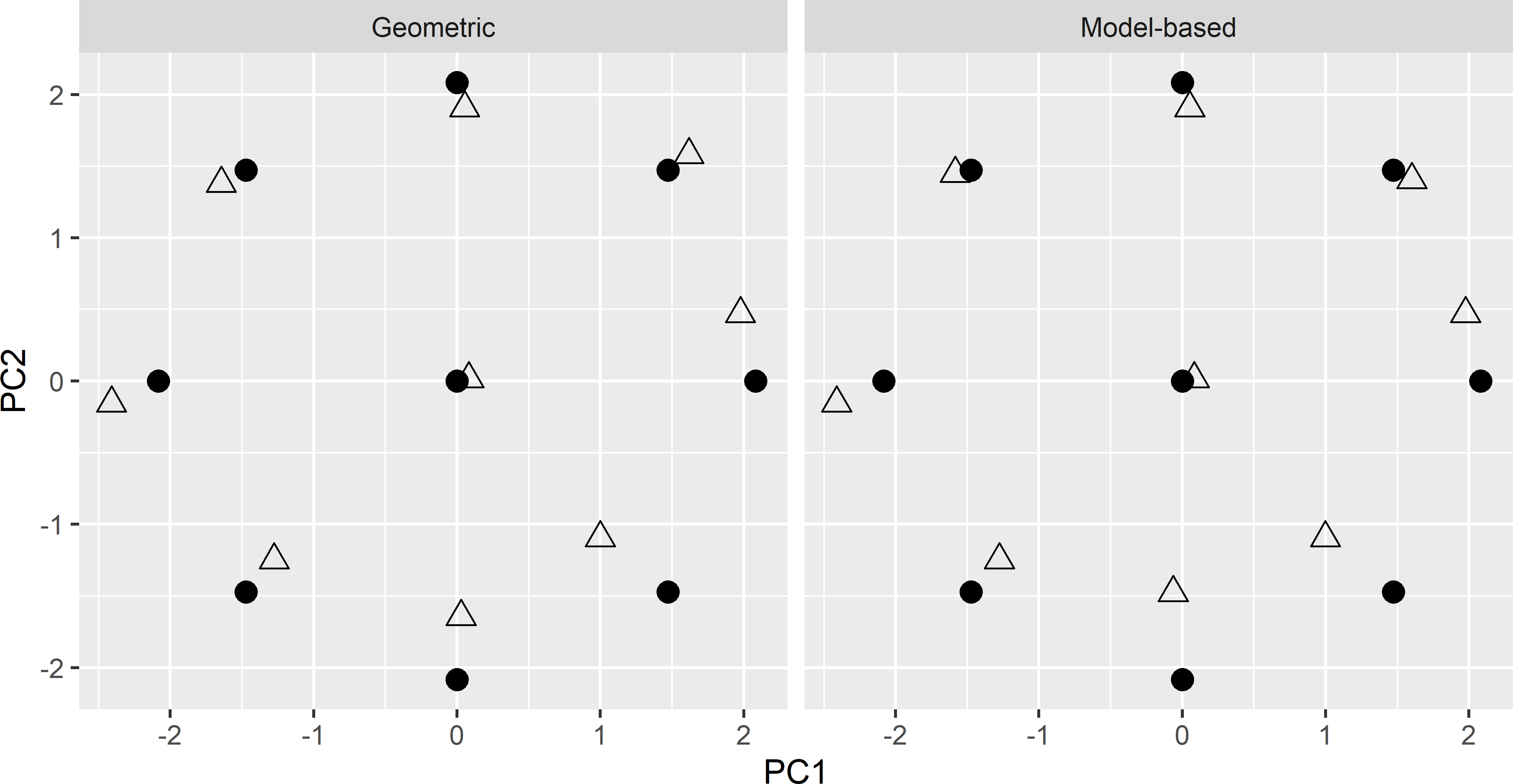
Figure 20.6: Principal component scores of the spatial CCRSD sample (triangles), optimised with the geometric and the model-based criterion. Dots: design points of CCRSD.
Figure 20.7 shows the two optimised CCRSD samples plotted in geographical space on the first standardised principal component scores.
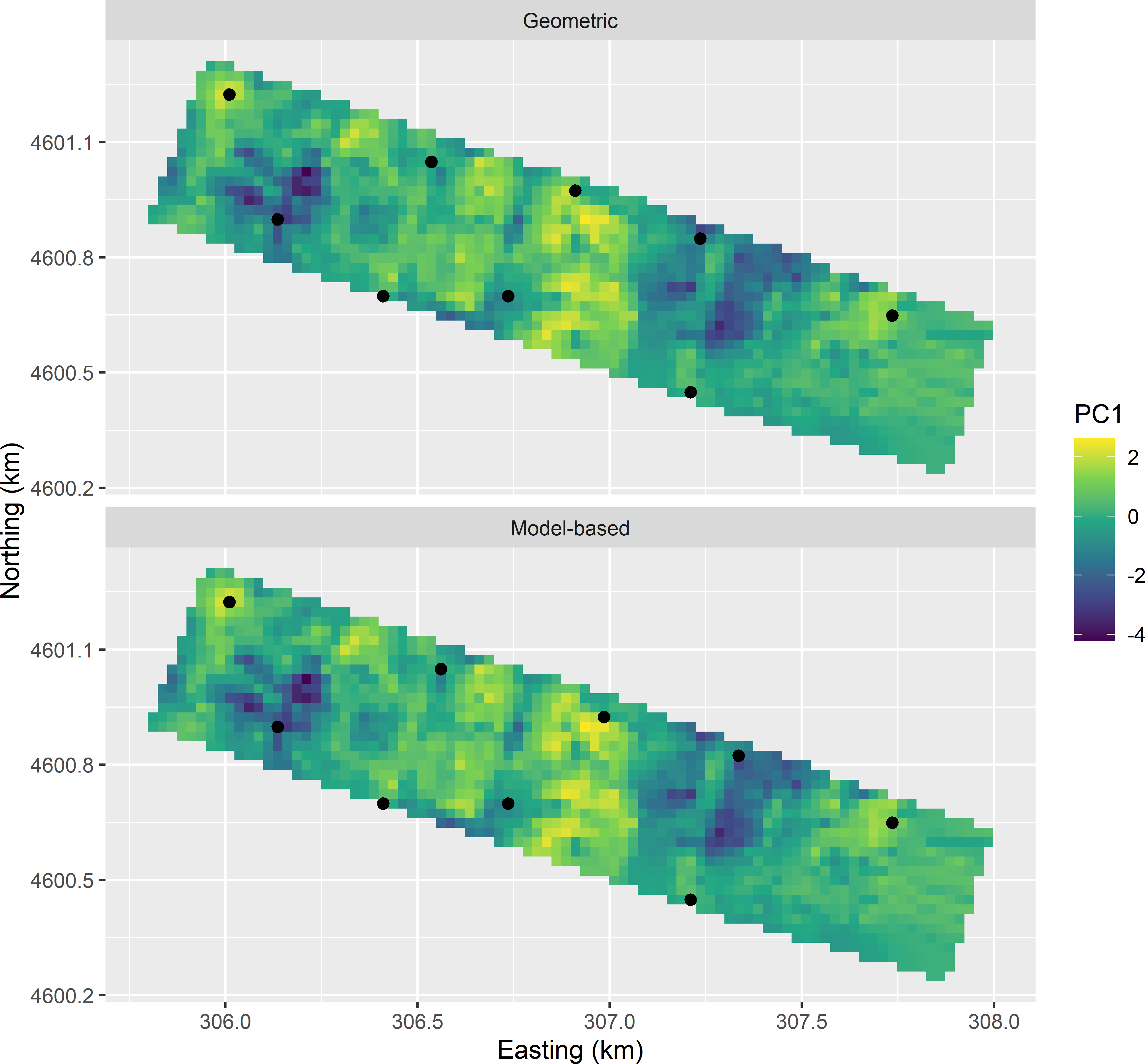
Figure 20.7: CCRSD sample from the Cotton Research Farm, optimised with the geometric and the model-based criterion, plotted on a map of the first standardised principal component (PC1).
20.1 Increasing the sample size
Nine points are rather few for fitting a polynomial regression model, especially for a second-order polynomial with interaction. Therefore, in experiments often multiple observations are done for each design point. Increasing the sample size of a response surface sample in observational studies is not straightforward. The challenge is to avoid spatial clustering of sampling points. A simple solution is to select multiple points from each subset of candidate sampling units. The success of this solution depends on how strong candidate sampling units are spatially clustered. For the Cotton Research Farm for most design points the candidate sampling units are not in one spatial cluster; so in this case, the solution may work properly. I increased the number of candidate sampling units per design point to 16, so that there is a larger choice in the optimisation of the sampling pattern.
candi_all <- NULL
for (i in seq_len(nrow(ccd_df))) {
    d2dpnt <- sqrt((grdCRF$PC1 - ccd_df$x1[i])^2 +
      (grdCRF$PC2 - ccd_df$x2[i])^2)
    grdCRF <- grdCRF[order(d2dpnt), ]
    candi <- grdCRF[c(1:16), c("point_id", "x", "y", "PC1", "PC2")]
    candi$dpnt <- i
    candi_all <- rbind(candi_all, candi)
}
A stratified simple random subsample of two points per stratum is selected, which serves as an initial sample.
set.seed(314)
units_stsi <- sampling::strata(
  candi_all, stratanames = "dpnt", size = rep(2, 9))
mysample0 <- getdata(candi_all, units_stsi) %>%
  dplyr::select(-(ID_unit:Stratum))
The data frame with the design points must be doubled. Note that the order of the design points must be equal to the order in the stratified subsample.
tmp <- data.frame(ccd_df, dpnt = 1:9)
ccd_df2 <- rbind(tmp, tmp)
ccd_df2 <- ccd_df2[order(ccd_df2$dpnt), ]
Figures 20.8 and 20.9 show the optimised CCRSD sample of 18 points in geographical and principal component space, respectively, obtained with the model-based criterion, an effective range of 150 m, and zero weight for the penalty term. Sampling points are not spatially clustered, so I do not expect violation of the assumption of independent residuals. In principal component space, all points are pretty close to the design points, except for the four design points in the lower right corner, where no candidate units near these design points are available.
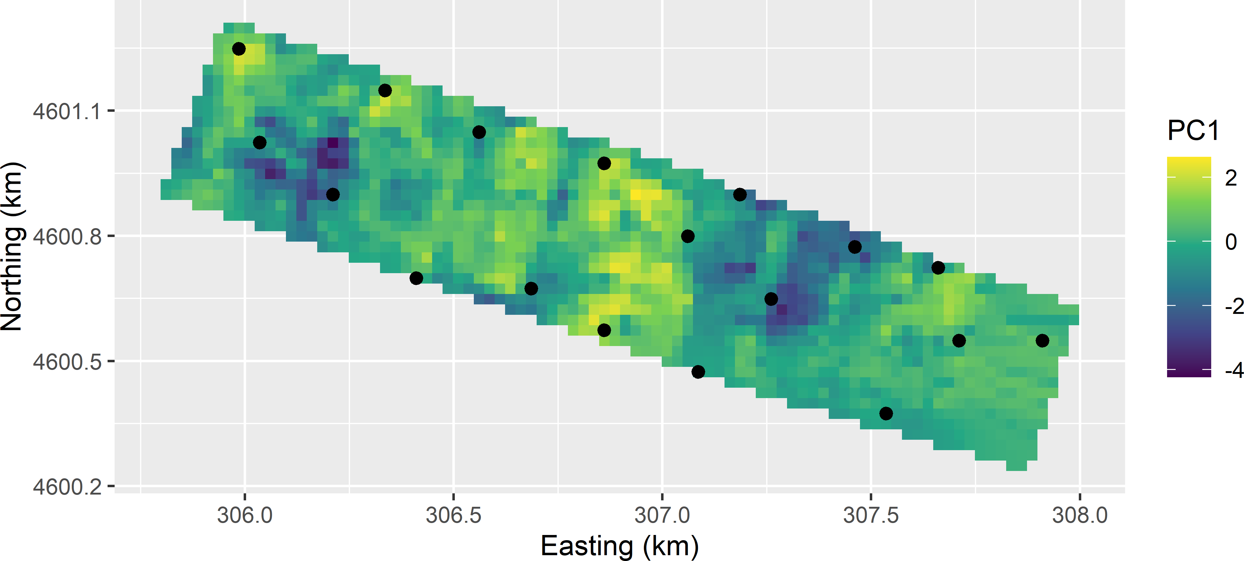
Figure 20.8: CCRSD sample with two points per design point, from the Cotton Research Farm, plotted on a map of the first standardised principal component (PC1).
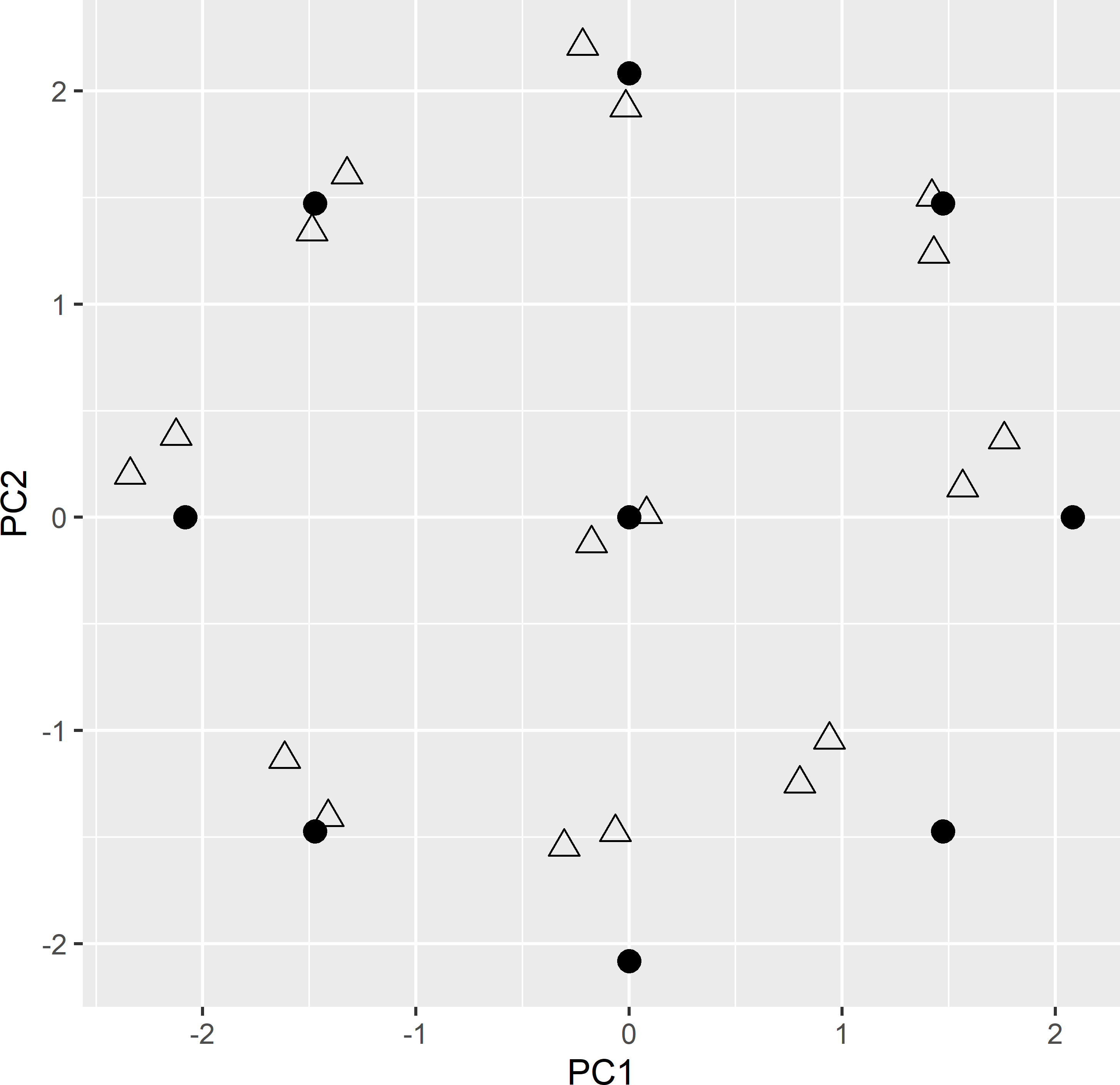
Figure 20.9: CCRSD sample (triangles) with two points per design point (dots), optimised with model-based criterion, plotted in the space spanned by the two standardised principal components.
20.2 Stratified spatial response surface sampling
The sample size can also be increased by stratified spatial response surface sampling. The strata are subareas of the study area. When the subsets of candidate sampling units for some design points are strongly spatially clustered, the final optimised sample obtained with the method of the previous section may also show strong spatial clustering. An alternative is then to split the study area into two or more subareas (strata) and to select from each stratum candidate sampling units. This guarantees that for each design point we have at least as many spatial clusters of candidate units as we have strata.
Figure 20.10 shows two subareas used as strata in stratified response surface sampling of the Cotton Research Farm.
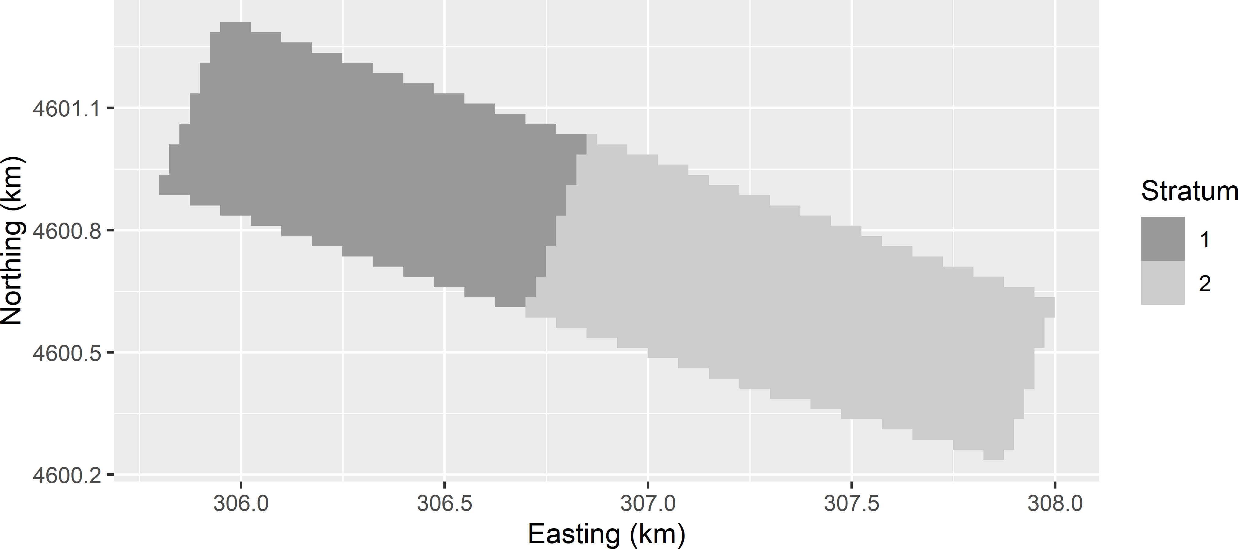
Figure 20.10: Two subareas of the Cotton Research Farm used as strata in stratified CCRSD sampling.
The candidate sampling units are selected in a double for-loop. The outer loop is over the strata, the inner loop over the design points. Note that variable dpnt continues to increase by 1 after the inner loop over the nine design points in subarea 1 is completed, so that variable dpnt (used as a stratification variable in subsampling the sample of candidate sampling points) now has values \(1,2, \dots , 18\). An equal number of candidate sampling points per design point in both strata (eight points) is selected by sorting the points of a stratum by the distance to a design point using function order. Figure 20.11 shows the candidate sampling points for stratified CCRSD sampling.
candi_all <- NULL
for (h in c(1, 2)) {
  data_stratum <- grdCRF %>%
    filter(subarea == h)
  candi_stratum <- NULL
  for (i in seq_len(nrow(ccd_df))) {
      d2dpnt <- sqrt((data_stratum$PC1 - ccd_df$x1[i])^2 +
                     (data_stratum$PC2 - ccd_df$x2[i])^2)
      data_stratum <- data_stratum[order(d2dpnt), ]
      candi <- data_stratum[c(1:8),
          c("point_id", "x", "y", "PC1", "PC2", "subarea")]
      candi$dpnt <- i + (h - 1) * nrow(ccd_df)
      candi_stratum <- rbind(candi_stratum, candi)
  }
  candi_all <- rbind(candi_all, candi_stratum)
}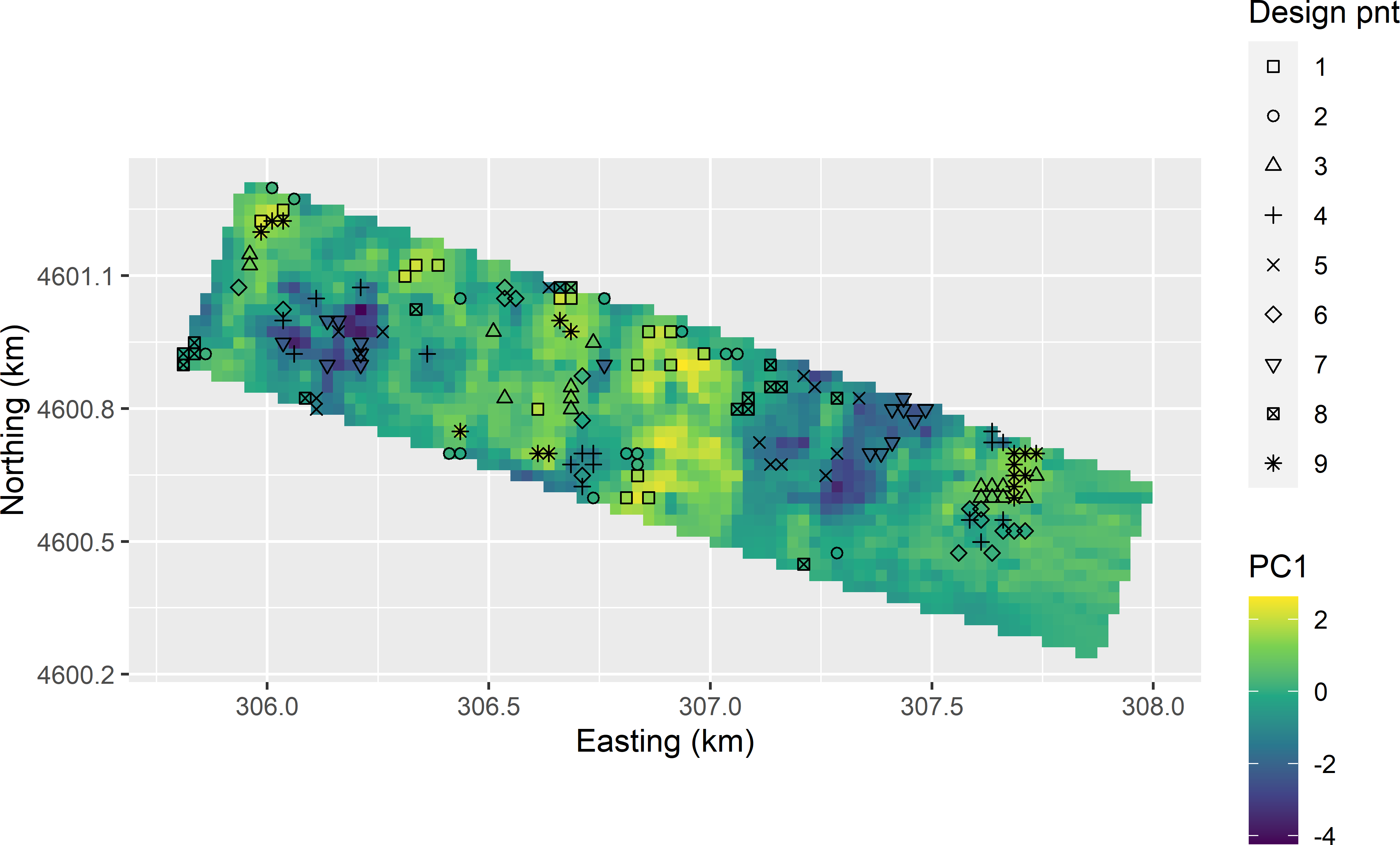
Figure 20.11: Candidate sampling points for stratified CCRSD sampling, plotted on a map of the first principal component (PC1).
As before, dpnt is used as a stratum identifier to subsample the candidate sampling units. Finally, the number of rows in data.frame ccd_df with the design points is doubled.
set.seed(314)
units_stsi <- sampling::strata(
  candi_all, stratanames = "dpnt", size = rep(1, 18))
mysample0 <- getdata(candi_all, units_stsi) %>%
  dplyr::select(-(ID_unit:Stratum))
ccd_df2 <- rbind(ccd_df, ccd_df)
Figures 20.12 and 20.13 show the optimised sample of 18 points in geographical and principal component space, obtained with the model-based criterion with an effective range of 150 m. The pattern in the principal component space is worse compared to the pattern in Figure 20.9. In stratum 1, the distance to the star point at the top and the upper left and upper right cube points is very large. In this stratum no population units are present that are close to these design points. By adding a penalty term to the minimisation criterion that is proportional to the distance to the design points, the distance is somewhat decreased, but not really for the three design points mentioned above (Figure 20.9). Also note the spatial cluster of three sampling units in Figure 20.12 obtained with a weight equal to 5.

Figure 20.12: Stratified CCRSD samples from the Cotton Research Farm, optimised with the model-based criterion, obtained without (weight = 0) and with penalty (weight = 5) for a large average distance to design points.
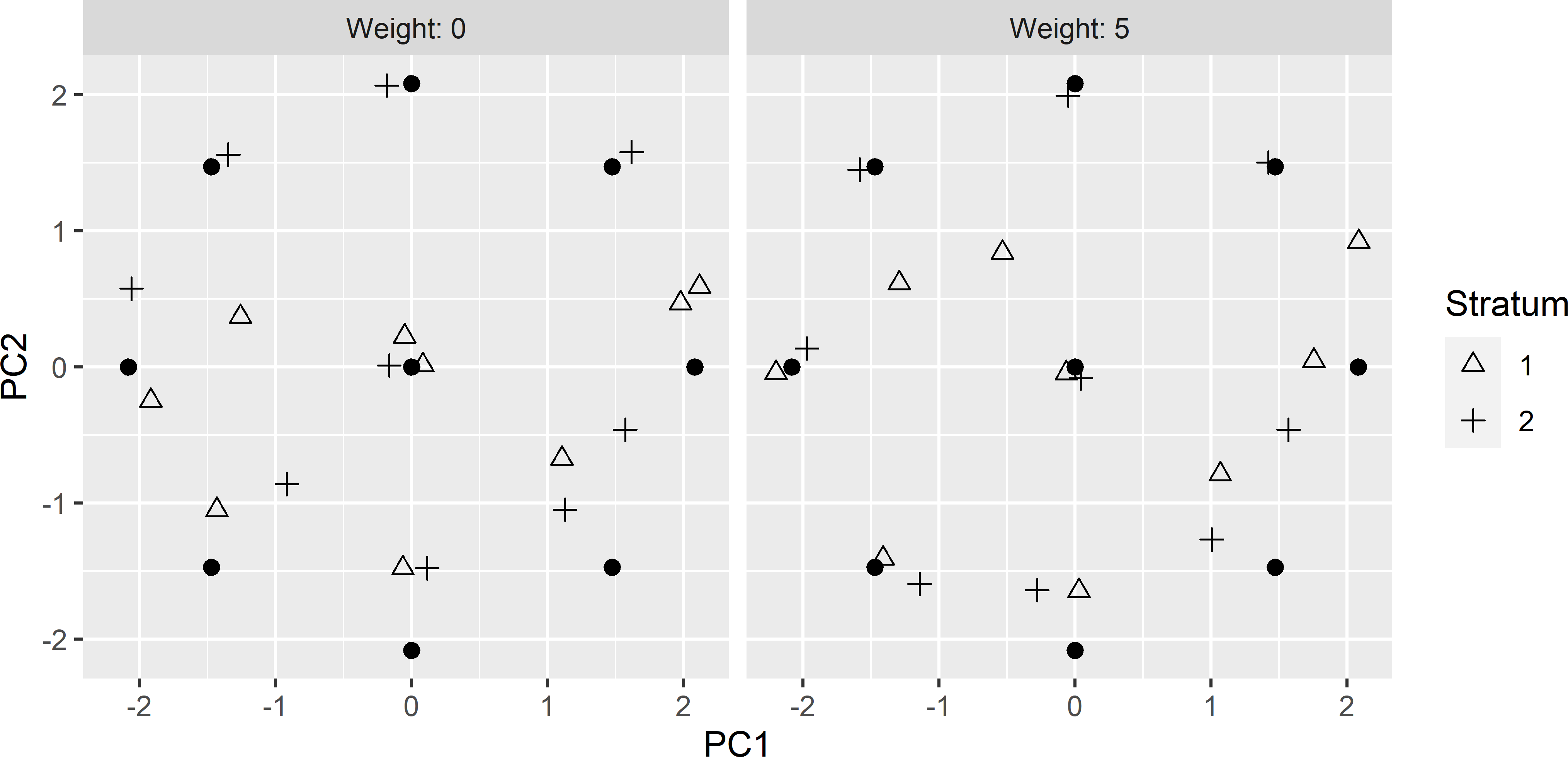
Figure 20.13: Principal component scores of the stratified CCRSD sample, optimised with the model-based criterion, obtained without (weight = 0) and with penalty (weight = 5) for a large average distance to design points (dots).
20.3 Mapping
Once the data are collected, the study variable is mapped by fitting a multiple linear regression model using the two covariates, in our case the two EM measurements, as predictors. The fitted model is then used to predict the study variable for all unsampled population units.
The value of the study variable at an unsampled prediction location \(\mathbf{s}_0\) is predicted by \[\begin{equation} \widehat{Z}(\mathbf{s}_0) = \mathbf{x}_0 \hat{\pmb{\beta}}_{\text{OLS}}\;, \tag{20.1} \end{equation}\] with \(\mathbf{x}_0\) the (\(p+1\))-vector with covariate values at prediction location \(\mathbf{s}_0\) and 1 in the first entry (\(p\) is the number of covariates) and \(\hat{\pmb{\beta}}\) the vector with ordinary least squares estimates of the regression coefficients: \[\begin{equation} \hat{\pmb{\beta}}_{\text{OLS}} = (\mathbf{X}^{\mathrm{T}}\mathbf{X})^{-1} (\mathbf{X}^{\mathrm{T}}\mathbf{z})\;, \tag{20.2} \end{equation}\] with \(\mathbf{X}\) the \((n \times (p+1))\) matrix with covariate values and ones in the first column (\(n\) is the sample size, and \(p\) is the number of covariates) and \(\mathbf{z}\) the \(n\)-vector with observations of the study variable.
The variance of the prediction error can be estimated by \[\begin{equation} \widehat{V}(\widehat{Z}(\mathbf{s}_0)) = \hat{\sigma}^2_{\epsilon}(1+\mathbf{x}_0^{\mathrm{T}}(\mathbf{X}^{\mathrm{T}}\mathbf{X})^{-1}\mathbf{x}_0)\;, \tag{20.3} \end{equation}\] with \(\hat{\sigma}^2_{\epsilon}\) the estimated variance of the residuals.
In R the model can be calibrated with function lm, and the predictions can be obtained with function predict. The standard errors of the estimated means can be obtained with argument se.fit = TRUE. The variances of Equation (20.3) can be computed by squaring these standard errors and adding the squared value of the estimated residual variance, which can be extracted with sigma().
mdl <- lm(lnECe ~ lnEM100cm + lnEM50cm, data = mysample)
zpred <- predict(mdl, newdata = grdCRF, se.fit = TRUE)
v_zpred <- zpred$se.fit^2+sigma(mdl)^2
The assumption underlying Equations (20.2) and (20.3) is that the model residuals are independent. We assume that all the spatial structure of the study variable is explained by the covariates. Even the residuals at two locations close to each other are assumed to be uncorrelated. A drawback of the spatial response surface design is that it is hard or even impossible to check this assumption, as the sampling locations are spread throughout the study area. If the residuals are not independent, the covariance of the residuals can be accounted for by generalised least squares estimation of the regression coefficients (Equation (21.24)). The study variable can then be mapped by kriging with an external drift (Section 21.3). However, this requires an estimate of the semivariogram of the residuals (Section 21.5).