Chapter 1 Introduction
This book is about sampling for spatial surveys. A survey is an inventory of an object of study about which statistical statements will be made based on data collected from that object. The object of study is referred to as the population of interest or target population. Examples are a survey of the organic carbon stored in the soil of a country, the water quality of a lake, the wood volume in a forest, the yield of rice in a country, etc. In these examples, soil organic carbon, water quality, wood volume, and rice yield are the study variables, i.e., the variables of which we want to estimate the population mean or some other parameter, or which we want to map. So, this book is about observational research, not about experiments. In experiments, observations are done under controlled circumstances; think of an experiment on crop yields as a function of application rates of fertiliser. Several levels of fertiliser application rate are chosen and randomly assigned to experimental plots. In observational research, factors that influence the study variable are not controlled. This implies that in observational research no conclusions can be drawn on causal relations.
If the whole population is observed, this is referred to as a census. In general, we cannot afford such a census. Only some parts of the population are selected and the study variable is observed (measured) for these selected parts (the population units in the sample) only. Such a survey is referred to as a sample survey. The observations are subsequently used to derive characteristics of the whole population. For instance, to estimate the wood volume in a forest, we cannot afford to measure the wood volume of every tree in the forest. Instead, some trees are selected, the wood volume of these trees is measured, and based on these measurements the total wood volume in the forest is estimated.
1.1 Basic sampling concepts
In this book the populations of interest have a spatial dimension. In selecting parts of such populations for observation, we may account for the spatial coordinates of the parts, but this is not strictly needed. Examples of spatial sampling designs are designs selecting sampling units that are spread throughout the study area, often leading to more precise estimates of the population mean or total as compared to sampling designs resulting in spatial clusters of units.
Two types of populations can be distinguished: discrete and continuous populations. Discrete populations consist of discrete natural objects, think of trees, agricultural fields, lakes, etc. These objects are referred to as population units. The total number of population units in a discrete population is finite. A finite spatial population of discrete units can be denoted by \(\mathcal{U}=\{u(\mathbf{s}_1),u(\mathbf{s}_2), \dots , u(\mathbf{s}_N)\}\), with \(u(\mathbf{s}_k)\) the unit located at \(\mathbf{s}_k\), where \(\mathbf{s}\) is a vector with spatial coordinates. The population units naturally serve as the elementary sampling units. In this book the spatial populations are two-dimensional, so a vector \(\mathbf{s}\) has two coordinates, Easting and Northing.
Other populations may, for the purpose of sampling, be considered as a physical continuum, e.g., the soil in a region, the water in a lake, the crop on a field.
Such continuous spatial populations can be denoted by \(\mathcal{U}=\{u(\mathbf{s}), \mathbf{s} \in \mathcal{A} \}\), with \(\mathcal{A}\) the study area. Discrete objects that can serve as elementary sampling units do not exist in continuous populations. Therefore, we must define the elementary sampling units. The elementary sampling units can be areal units, e.g., 10 m squares; or circular plots, e.g., with a radius of 5 m; or “points”, i.e., units of such a small area, compared to the area of the population, that the area of the units can be ignored.
In this book a population unit and an elementary sampling unit can be an individual object of a discrete population as well as an areal sampling unit or a point of a continuous population.
The size and geometry of the elementary units used in sampling a continuous population is referred to as the sample support. The total number of elementary sampling units in a continuous population can be finite, e.g., all 25 m \(\times\) 25 m (disjoint) raster cells in an area (raster cells in Figure 1.1), or infinite, e.g., all points in an area, or all squares or circular plots with a given radius that are allowed to overlap in an area (circles in Figure 1.1).
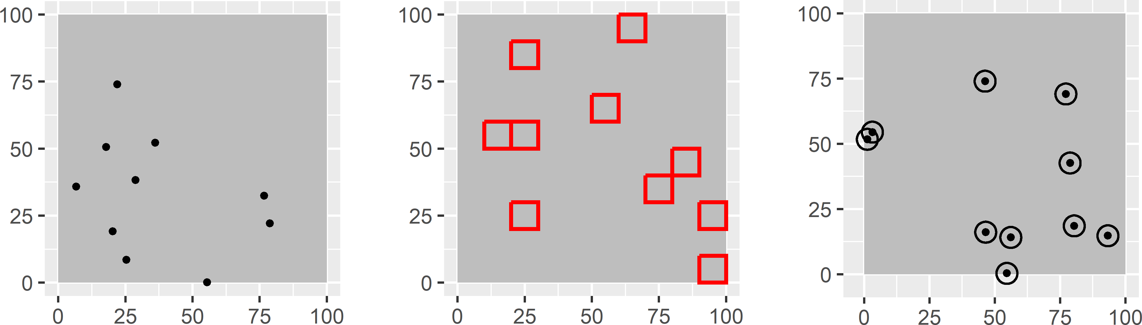
Figure 1.1: Three sample supports: points, squares, and circles. With disjoint squares, the population is finite. With points, and squares or circles that are allowed to overlap, the population is infinite.
Ideally, with areal elementary sampling units, the selected elementary units are exhaustively observed, so that a measurement of the total or mean of the study variable within an areal unit is obtained, think for instance of the total aboveground biomass. In some cases this is not feasible, think for instance of measuring the mean of some soil property in 25 m squares. In this case, a sample of points is selected from each selected square, and the measurement is done at the selected points. These measurements at points are used to estimate the mean of the squares. Stehman et al. (2018) introduced the concept of a response design as “the protocol used to determine the reference condition of an element of the population”. So, in the case just mentioned the response design is the sampling design and the estimator for the mean of the soil property of the 25 m squares.
Ideally, the sample support is constant, but in some situations a varying sample support cannot be avoided. Think, for instance, of square sampling units in an irregularly shaped study area. Near the border of the study area, there are squares that cross the border. The part of a square that falls outside the study area is not observed. So, the support of the observations of squares crossing the border is smaller than that of the observations of squares in the interior of the study area. See also Section 3.4.
To sample a finite spatial population, the population units are listed in a data frame. This data frame contains the spatial coordinates of the population units and other information needed for selecting sampling units according to a specific design. Think, for instance, of the labels of more or less homogeneous subpopulations (used as strata in stratified random sampling, see Chapter 4) and the labels of clusters of population units, for instance, all units in a polygon of a map (used in cluster random sampling, see Chapter 6). Besides, if we have information about covariates possibly related to the study variable, which we would like to use in selecting the population units, these covariates are added to the list. The list used for selecting sampling units is referred to as the sampling frame.
If the elementary sampling units are disjoint square grid cells (sample support is a square), the population is finite and the grid cells can be selected through selection of their centres (or any other point that uniquely identifies a grid cell) listed in the sampling frame.
In this book also continuous populations are sampled using a list as a sampling frame. The infinite population is discretised by the cells of a fine discretisation grid. The grid cells are listed in the sampling frame by the spatial coordinates of the centres of the grid cells. So, the infinite population is represented by a finite list of points. The advantage of this is that existing R packages for sampling of finite populations can also be used for sampling infinite populations.
If the elementary sampling units are points (sample support is a point), the population is infinite. In this case, sampling of points can be implemented by a two-step approach. In the first step, cells of the discretisation grid are selected with or without replacement, and in the second step one or more points are selected within the selected grid cells. Figure 1.2 is an illustration of this two-step approach for simple random sampling of points from a discretised infinite population. Ten grid cells are selected by simple random sampling with replacement. Every time a grid cell is selected, one point is randomly selected from that grid cell. Note that a grid cell can be selected more than once, so that more than one point will be selected from that grid cell. Note also that we may select a point that falls outside the boundary of the study area. This is actually the case with one grid cell in Figure 1.2. The points outside the study area are discarded and replaced by a randomly selected new point inside the study area. Finally, note that near the boundary there are small areas not covered by a grid cell, so that no points can be selected in these areas. It is important that the discretisation grid is fine enough to keep the discretisation error so small that it can be ignored. The alternative is to extend the discretisation grid beyond the boundaries of the study area so that the full study area is covered by grid cells.
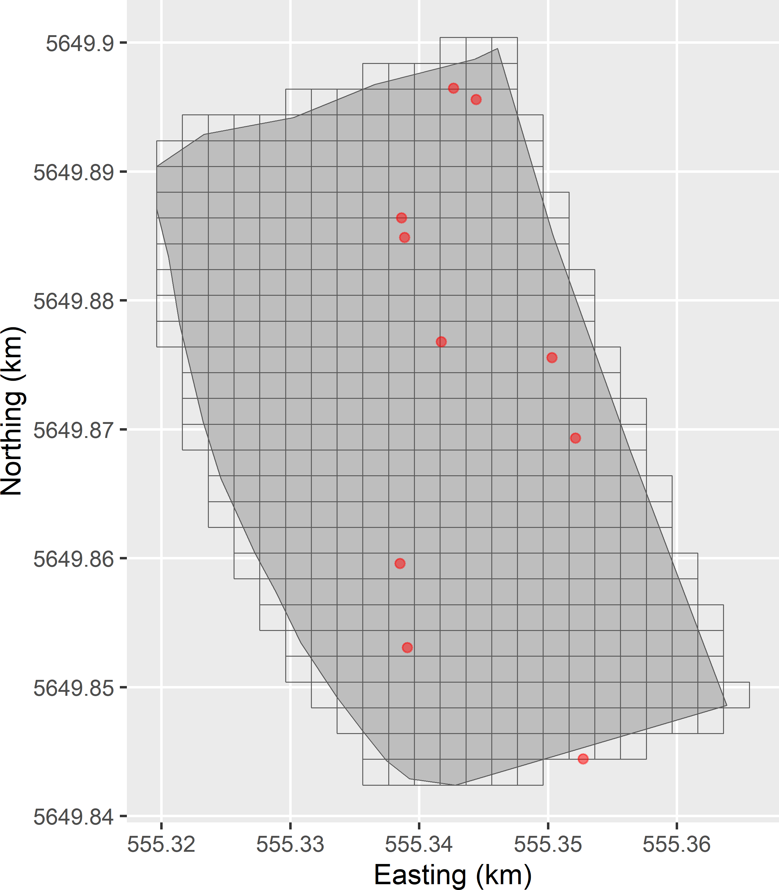
Figure 1.2: Sampling of points from discretised infinite population. The grid cells are randomly selected with replacement. Each time a grid cell is selected, a point is randomly selected from that grid cell.
1.1.1 Population parameters
The sample data are used to estimate characteristics of the whole population, e.g., the population mean or total; some quantile, e.g., the median or the 90th percentile; or even the entire cumulative frequency distribution.
A finite population total is defined as
\[\begin{equation} t(z) = \sum_{k \in \mathcal{U}} z_k = \sum_{k=1}^N z_k \;, \tag{1.1} \end{equation}\]
with \(N\) the number of population units and \(z_k\) the study variable for population unit \(k\). A finite population mean is defined as a finite population total divided by \(N\).
An infinite population total is defined as an integral of the study variable over the study area:
\[\begin{equation} t(z) = \int_{\mathbf{s} \in \mathcal{A}} z(\mathbf{s}) \;\mathrm{d}\mathbf{s} \;. \tag{1.2} \end{equation}\]
An infinite population mean is defined as a finite population total divided by the area, \(A\), covered by the population.
A finite population proportion is defined as the population mean of an 0/1 indicator \(y\) with value 1 if the condition is satisfied, and 0 otherwise:
\[\begin{equation} p=\frac{\sum_{k=1}^N y_k}{N} \;. \tag{1.3} \end{equation}\]
A cumulative distribution function (CDF) is defined as
\[\begin{equation} F(z)=\sum_{z^\prime \leq z} p(z^\prime) \;, \tag{1.4} \end{equation}\]
with \(p(z^\prime)\) the proportion of population units whose value for the study variable equals \(z^\prime\).
A population quantile, for instance the population median or the population 90th percentile, is defined as
\[\begin{equation} q_p= F^{-1}(p) \;, \tag{1.5} \end{equation}\]
where \(p\) is a number between 0 and 1 (e.g., 0.5 for the median, 0.9 for the 90th percentile), and \(F^{-1}(p)\) is the smallest value of the study variable \(z\) satisfying \(F(z)\geq p\).
In surveys of spatial populations, the aim can also be to make a map of the population.
1.1.2 Descriptive statistics vs. inference about a population
When we observe only a (small) part of the population, we are uncertain about the population parameter estimates and the map of the population. By using statistical methods, we can quantify how uncertain we are about these results. In decision making it can be important to take this uncertainty into account. An example is a survey of water quality. In Europe the concentration levels of nutrients are regulated in the European Water Framework Directive. To test whether the mean concentration of a nutrient complies with its standard, it is important to account for the uncertainty in the estimated mean. When the estimated mean is just below the standard, there is still a large probability that the population mean exceeds the standard. This example shows that it is important to distinguish computing descriptive statistics from characterising the population using the sample data. For instance, we can compute the sample mean (average of the sample data) without error, but if we use this sample mean as an estimate of the population mean, there is certainly an error in this estimate.
1.1.3 Random sampling vs. probability sampling
Many sampling methods are available. At the highest level, one may distinguish random from non-random sampling methods. In random sampling, a subset of population units is randomly selected from the population, using a (pseudo) random number generator. In non-random sampling, no such random number generator is used. Examples of non-random sampling are (i) convenience sampling, i.e., sampling at places that are easy to access, e.g., along roads; (ii) arbitrary sampling, i.e., sampling without a specific purpose in mind; and (iii) targeted sampling, e.g., at sites suspected of soil pollution.
In the literature, the term is often used for arbitrary sampling, i.e., sampling without a specific purpose in mind. To avoid confusion the term probability sampling is used for random sampling using a (pseudo) random number generator, so that for any unit in the population the probability of selecting that unit is known. More precisely, a probability sample is a sample from a population such that every unit of the population has a positive probability of being included in the sample. Besides, these inclusion probabilities must be known, at least for the selected units, as they are needed in estimation. This is explained in following chapters.
1.2 Design-based vs. model-based approach
The choice between probability or non-probability sampling is closely connected with the choice between the design-based or the model-based approach for sampling and statistical inference (estimation, hypothesis testing). The difference between these two approaches is a rather technical subject, so, not to discourage you already in this very first chapter, I will keep it short. In Chapter 26 I elaborate on the fundamental difference of these two approaches and a third approach, the model-assisted approach, which can be seen as a compromise of the design-based and the model-based approach.
| Approach | Sampling | Inference |
|---|---|---|
| Design-based | Probability sampling required | Based on sampling distribution |
| (no model used) | ||
| Model-based | Probability sampling not required | Based on statistical model |
In the design-based approach, units are selected by probability sampling (Table 1.1). Estimates are based on the inclusion probabilities of the sampling units as determined by the sampling design (design-based inference). No model is used in estimation. On the contrary, in the model-based approach a statistical model is used in prediction, i.e., a model with a random error term, for instance a regression model. As the model already contains a random error term, probability sampling is not required in this approach.
Which statistical approach is best largely depends on the aim of the survey, see Brus and de Gruijter (1997) and de Gruijter et al. (2006). Broadly speaking, the following aims can be distinguished:
- estimating parameters for the population;
- estimating parameters for several subpopulations; and
- mapping the study variable.
When the aim is to map the study variable, a model-based approach is the most natural option. This implies that for this aim probability sampling is not necessarily required. In principle, both approaches are suitable for estimating (sub)population parameters. The more subpopulations are distinguished, the more attractive a model-based approach becomes. Model-based estimates of the subpopulation means or totals are potentially more accurate (depending on how good the model is) than model-free design-based estimates. On the other hand, an advantage of design-based estimation is that an objective assessment of the uncertainty of the estimated mean or total is warranted, and that the coverage of confidence intervals is (almost) correct.
A probability sample can also be used in model-based inference. This flexibility can be attractive when we have a dual aim, mapping as well as estimation of parameters of (sub)populations. When units are not selected by probability sampling, model-free design-based estimation is impossible, and model-based prediction is the only option.
1.3 Populations used in sampling experiments
In this book various data sets are used to illustrate the sampling designs. Four data sets, Voorst, Kandahar, Eastern Amazonia, and the Iberian Peninsula (Spain and Portugal), are exhaustive, i.e., for all population units, data of the study variable and ancillary data are available. The first two exhaustive data sets are obtained through simulation, i.e., by drawing numbers from a probability distribution. Sample data from these two study areas are used to calibrate a statistical model. This model is subsequently used to simulate values of the study variable for all population units. Voorst actually is an infinite population of points. However, this study area is discretised by the cells of a fine grid, and the study variable, the soil organic matter (SOM) concentration, is simulated for all centres of the grid cells. Kandahar is a finite population consisting of 965 squares of size 5 km \(\times\) 5 km. The study variable is the area cultivated with poppy. Eastern Amazonia is a map in raster format, with a resolution of 1 km \(\times\) 1 km. The study variable is the aboveground biomass as derived from remote sensing images. The aboveground biomass value of a raster cell is treated as the average biomass of that raster cell. The data set Iberian Peninsula is a time series of four maps in raster format with a resolution of 30 arc sec. The study variable is the annual mean air temperature at two metres above the earth surface in \(^\circ\)C.
The exhaustive data sets are used in the first part of this book on probability sampling for estimating population parameters. By taking the population as the reality, we know the population parameters. Also, for any randomly selected sample from this population, the study variable values for the selected sampling units are known, so that we can estimate the population parameters from this sample. An estimated population parameter can then be compared with the population parameter. The difference between these two is the sampling error in the estimated population parameter. This opens up the possibility of repeating the random selection of samples with a given sampling design a large number of times, estimating the population parameter for every sample, so that a frequency distribution of the estimated population parameter is obtained. Ideally, the mean of this frequency distribution, referred to as the sampling distribution, is equal to the population parameter (mean sampling error equals zero), and the variance of the estimated population parameters is small. Another advantage is that sampling designs can be compared on the basis of the sampling distribution, for instance the sampling distributions of the estimator of the population mean with stratified random sampling and simple random sampling, to evaluate whether the stratification leads to more accurate estimates of the population mean.
Furthermore, various data sets are used with data for a sample of population units only. These data sets are described at places where they are first used.
All data sets are available by installing the R package sswr. This package can be installed from github with function install_github of package remotes (Csárdi et al. 2021).
The package can then be loaded. You can see the contents of the package and of the data files by typing a question mark, followed by the name of the package or a data file.
1.3.1 Soil organic matter in Voorst, the Netherlands
The study area of Voorst is located in the eastern part of the Netherlands. The size of the study area is 6 km \(\times\) 1 km. At 132 points, samples of the topsoil were collected by graduate students of Wageningen University, which were then analysed for SOM concentrations (in g kg-1 dry soil) in a laboratory. The map is created by conditional geostatistical simulation of natural logs of the SOM concentration on a 25 m \(\times\) 25 m grid, followed by backtransformation, using a linear mixed model with spatially correlated residuals and combinations of soil type and land use as a qualitative predictor (factor). Figure 1.3 shows the simulated map of the SOM concentration.
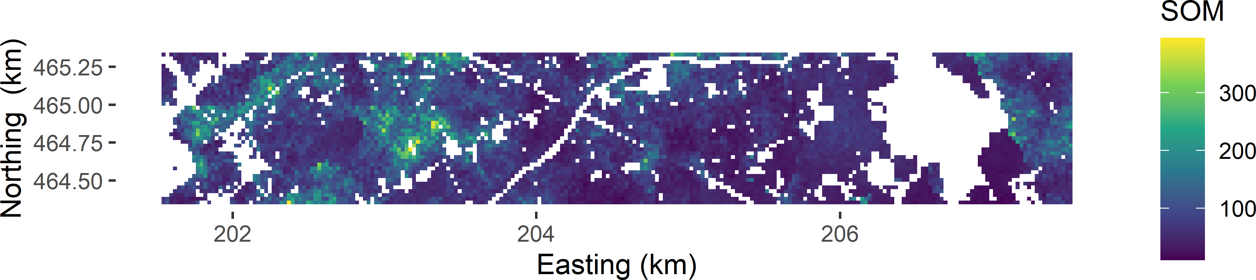
Figure 1.3: Simulated map of the SOM concentration (g kg-1) in Voorst.
The frequency distribution of the simulated values at all 7,528 grid cells shows that the SOM concentration is skewed to the right (Figure 1.4).
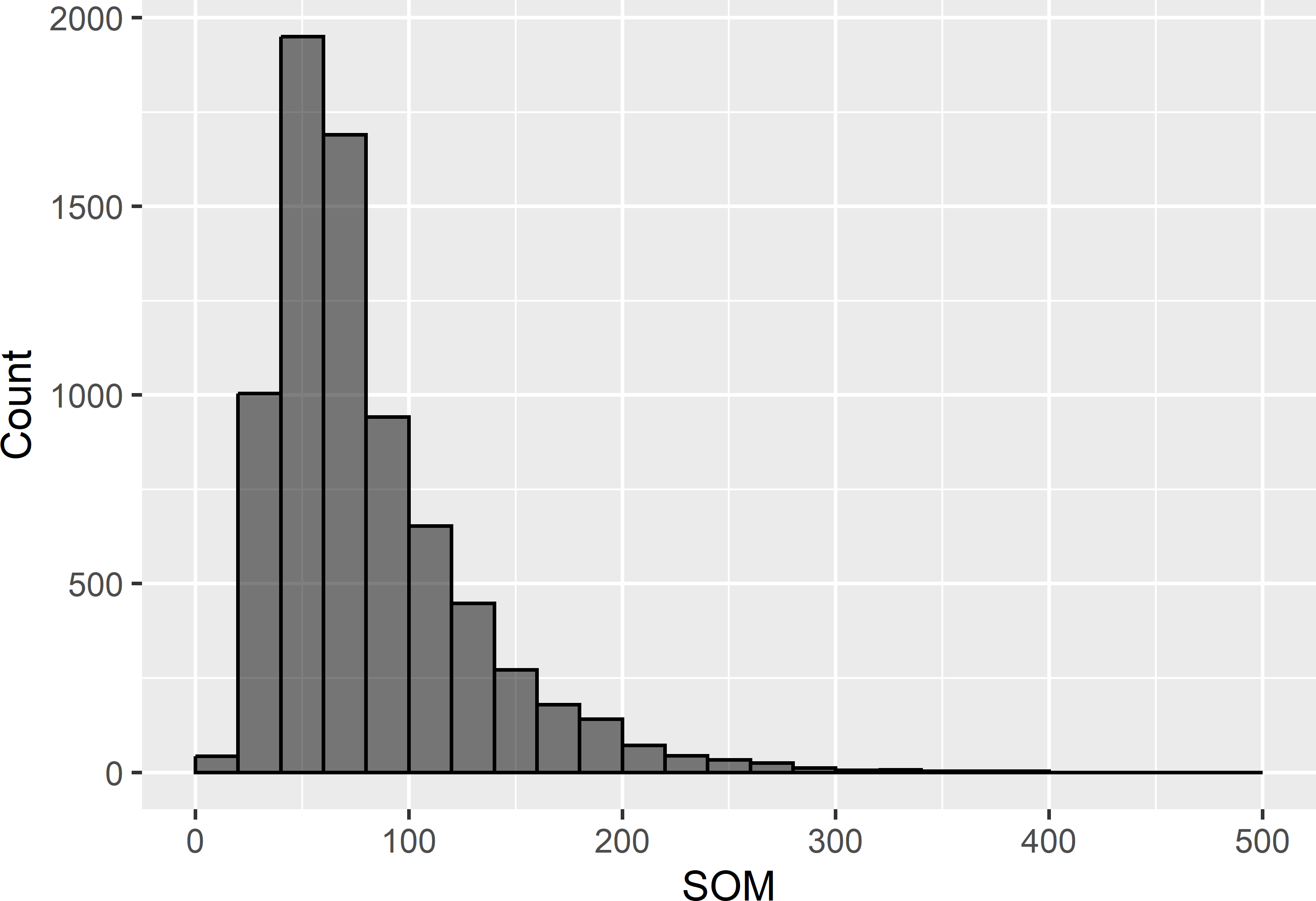
Figure 1.4: Frequency distribution of the simulated SOM concentration (g kg-1) in Voorst.
Summary statistics are:
   Min. 1st Qu.  Median    Mean 3rd Qu.    Max.
  10.75   49.45   68.15   81.13  100.63  394.45
The ancillary information consists of a map of soil classes and a land use map, which are combined to five soil-land use combinations (Figure 1.5). The first letter in the labels for the combinations stands for the soil type: B for beekeerdgrond (sandy wetland soil with gleyic properties), E for enkeerdgrond (sandy soil with thick anthropogenic humic topsoil), P for podzols (sandy soil with eluviated horizon below the topsoil), R for river clay soil, and X for other sandy soils. The second letter is for land use: A for agriculture (grassland, arable land) and F for forest.
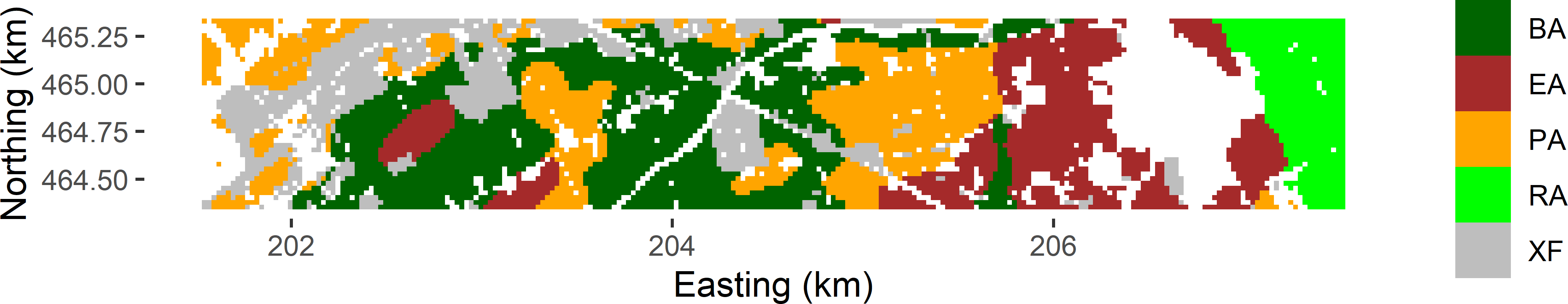
Figure 1.5: Soil-land use combinations in Voorst.
1.3.2 Poppy fields in Kandahar, Afghanistan
Cultivation of poppy for opium production is a serious problem in Afghanistan. The United Nations Office on Drugs and Crime (UNODC) monitors the area cultivated with poppy through detailed analysis of aerial photographs and satellite images. This is laborious, and therefore the analysis is restricted to a probability sample of 5 km squares. These sample data are then used to estimate the total poppy area (Anonymous 2014).
In 2014 the poppy area within 83 randomly selected squares in the province of Kandahar was determined, as well as the agricultural area within all 965 squares in this province. These data were used to simulate a map of poppy area per 5 km square. The map is simulated with an ordinary kriging model for the logit transform of the proportion of the agricultural area cultivated with poppy within 5 km squares. For privacy reasons, the field was simulated unconditionally on these sample data. Figure 1.6 shows the map with the agricultural area in hectares per 5 km square, and the map with the simulated poppy area in hectares per square. The frequency distribution of the simulated poppy area per square shows very strong positive skew (Figure 1.7). For 375 squares, the simulated poppy area was smaller than 1 hectare (ha).
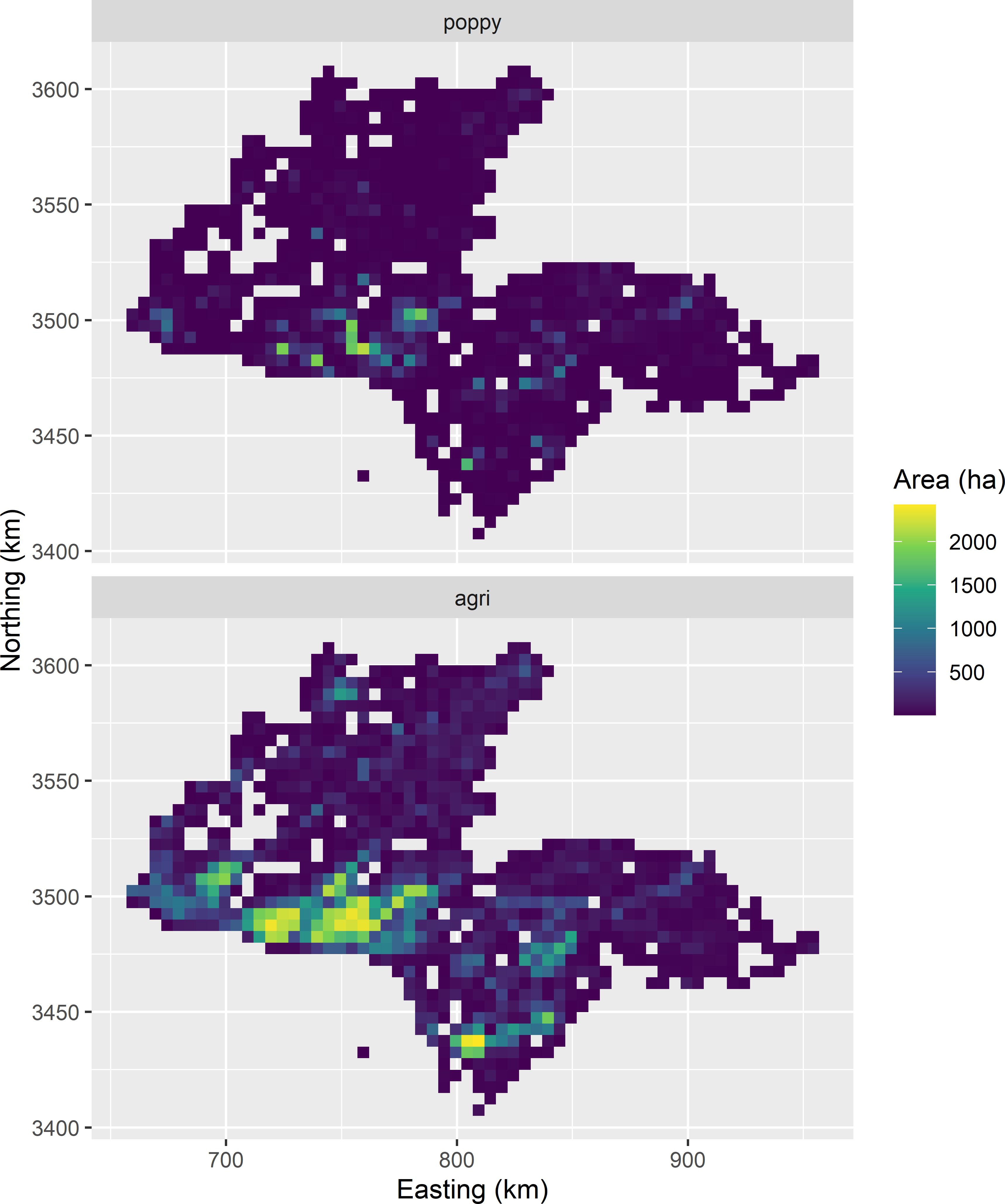
Figure 1.6: Agricultural area and simulated poppy area, in ha per 5 km square, in Kandahar.

Figure 1.7: Frequency distribution of simulated poppy area in ha per 5 km square, in Kandahar.
1.3.3 Aboveground biomass in Eastern Amazonia, Brazil
This data set consists of data on the live woody aboveground biomass (AGB) in megatons per ha (Baccini et al. 2012). A rectangular area of 1,642 km \(\times\) 928 km in Eastern Amazonia, Brazil, was selected from this data set. The data were aggregated to a map with a resolution of 1 km \(\times\) 1 km. Besides, a stack of five ecologically relevant covariates of the same spatial extent was prepared, being long term mean of MODIS short-wave infrared radiation (SWIR2), primary production in kg C per m2 (Terra_PP), average precipitation in driest month in mm (Prec_dm), elevation in m, and clay content in g kg-1 soil. All covariates were either resampled by bilinear interpolation or aggregated to conform with the grid of the aboveground biomass map. Figure 1.8 shows a map of AGB and SWIR2.
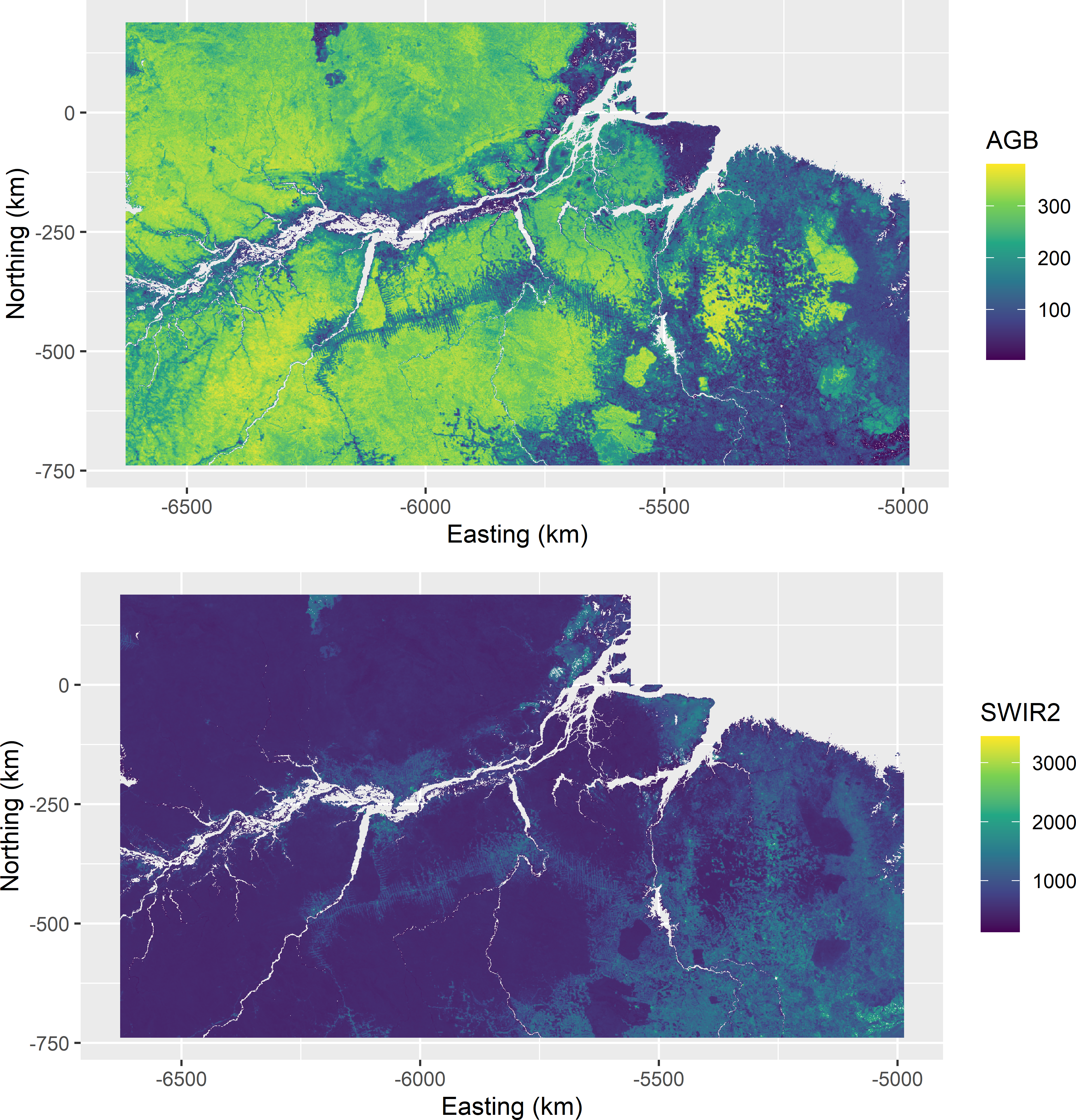
Figure 1.8: Aboveground biomass (AGB) in 109 kg ha-1 and short-wave infrared radiation (SWIR2) of Eastern Amazonia.
Figure 1.9 shows a matrix of two-dimensional density plots of aboveground biomass and the five covariates, made with function ggpairs of R package GGally (Schloerke et al. 2021). The covariate with the strongest correlation with AGB is SWIR2. The Pearson correlation coefficient with AGB is -0.80. The relation does not look linear. The correlation of AGB with the covariates Terra_PP and Prec_dm is weakly positive. All correlations are significant, but this is not meaningful because of the very large number of data used in computing the correlation coefficients.
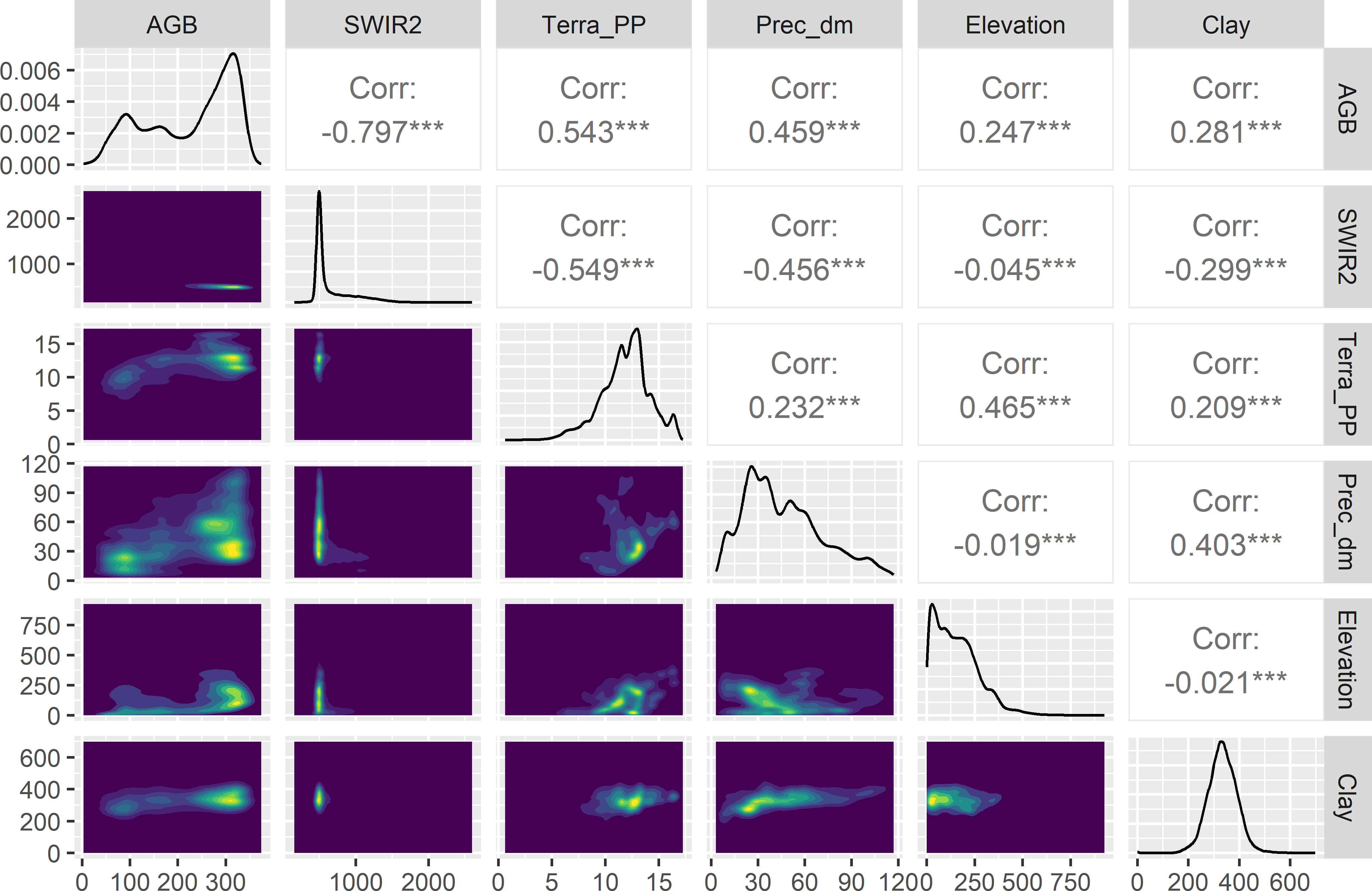
Figure 1.9: Matrix of two-dimensional density plots of AGB and five covariates of Eastern Amazonia. Terra_PP values are divided by 1000.
1.3.4 Annual mean air temperature in Iberia
The space-time designs of Chapter 15 are illustrated with the annual mean air temperature at two metres above the earth surface (TAS) in \(^\circ\)C, in Iberia (Spain and Portugal, islands excluded) for 2004, 2009, 2014, and 2019 (Figure 1.10). These data are part of the data set CHELSA (Karger et al. 2017). The raster files are latitude-longitude grids with a resolution of 30 arc sec. The data are projected using the Lambert azimuthal equal area (laea) projection. The resolution of the resulting laea raster file is about 780 m \(\times\) 780 m.
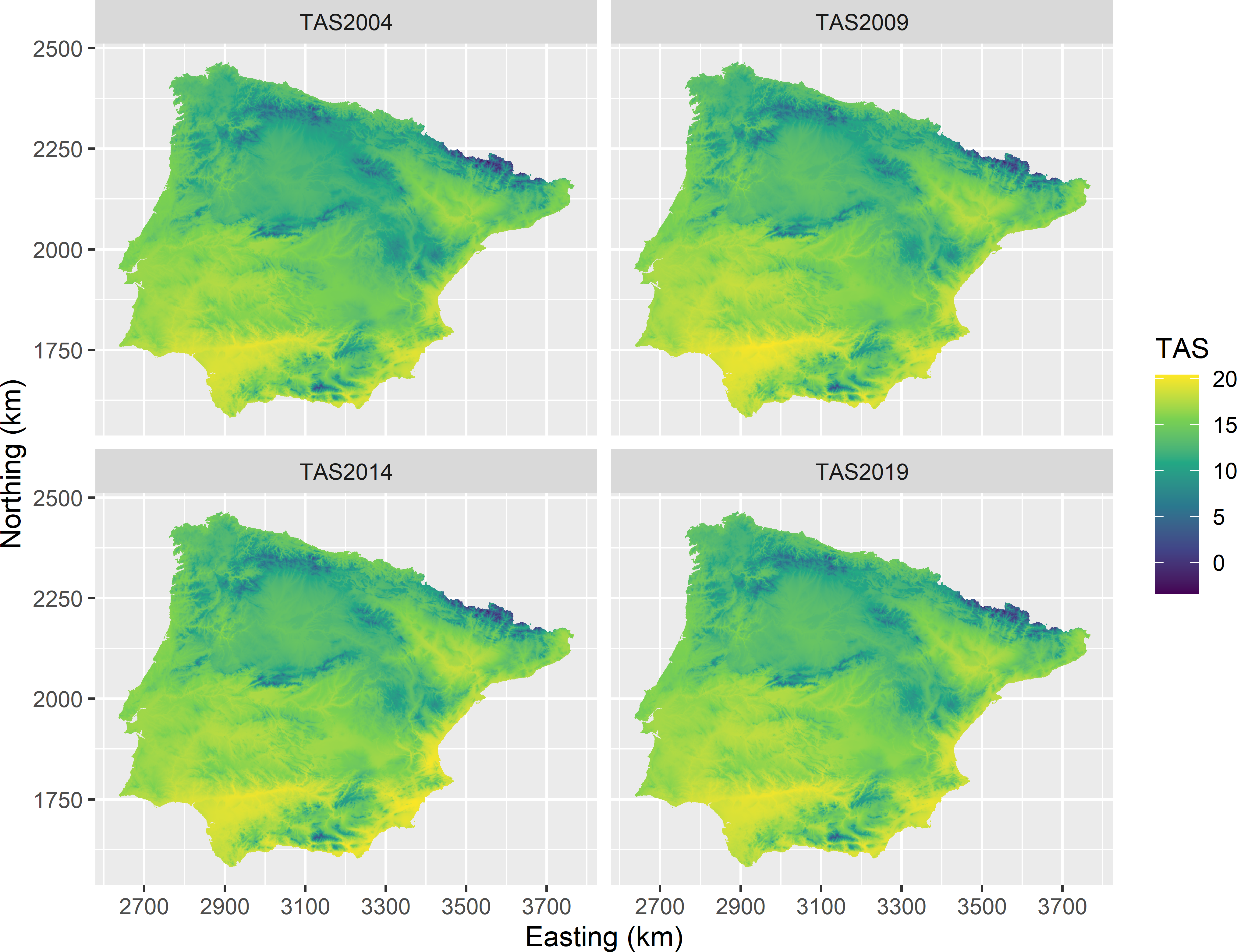
Figure 1.10: Annual mean air temperature in Iberia for 2004, 2009, 2014, and 2019.