Chapter 21 Introduction to kriging
In the following chapters a geostatistical model, i.e., a statistical model of the spatial variation of the study variable, is used to optimise the sample size and/or spatial pattern of the sampling locations. This chapter is a short introduction to geostatistical modelling.
In Chapter 13 we have already seen how a geostatistical model can be used to optimise probability sampling designs for estimating the population mean or total. In the following chapters, the focus is on mapping. A map of the study variable is obtained by predicting the study variable at the nodes of a fine discretisation grid. Spatial prediction using a geostatistical model is referred to as kriging (Webster and Oliver 2007).
With this prediction method, besides a map of the kriging predictions, a map of the variance of the prediction error is obtained. I will show hereafter that the prediction error variance is not influenced by the values of the study variable at the sampling locations. For this reason, it is possible to search, before the start of the survey, for the sampling locations that lead to the minimum prediction error variance averaged over all nodes of a fine prediction grid, provided that the geostatistical model is known up to some extent.
21.1 Ordinary kriging
The kriging predictions and prediction error variances are derived from a statistical model of the spatial variation of the study variable. There are several versions of kriging, but most of them are special cases of the following generic model:
\[\begin{equation} \begin{split} Z(\mathbf{s}) &= \mu(\mathbf{s}) + \epsilon(\mathbf{s}) \\ \epsilon(\mathbf{s}) &\sim \mathcal{N}(0,\sigma^2) \\ \mathrm{Cov}(\epsilon(\mathbf{s}),\epsilon(\mathbf{s}^{\prime})) &= C(\mathbf{h})\;, \end{split} \tag{21.1} \end{equation}\]
with \(Z(\mathbf{s})\) the study variable at location \(\mathbf{s}\), \(\mu(\mathbf{s})\) the mean at location \(\mathbf{s}\), \(\epsilon(\mathbf{s})\) the residual (difference between study variable \(z\) and mean \(\mu(\mathbf{s})\)) at location \(\mathbf{s}\), and \(C(\mathbf{h})\) the covariance of the residuals at two locations separated by vector \(\mathbf{h} = \mathbf{s} - \mathbf{s}^{\prime}\).
In ordinary kriging (OK) it is assumed that the mean of the study variable is constant, i.e., the same everywhere (Webster and Oliver 2007):
\[\begin{equation} Z(\mathbf{s}) = \mu + \epsilon(\mathbf{s}) \;, \tag{21.2} \end{equation}\]
with \(\mu\) the constant mean, independent of the location \(\mathbf{s}\). Stated otherwise, in OK we assume stationarity in the mean over the area to be mapped.
\(C(\cdot)\) is the covariance function, also referred to as the covariogram, and a scaled version of it, obtained by dividing \(C(\cdot)\) by the variance \(C(0)\), is the correlation function or correlogram.
If the data set is of substantial size, it is possible to define a neighbourhood: not all sample data are used to predict the study variable at a prediction location, but only the sample data in this neighbourhood. This implies that the stationarity assumption is relaxed to the often more realistic assumption of a constant mean within neighbourhoods.
In OK, the study variable at a prediction location \(\mathbf{s}_0\), \(\widehat{Z}(\mathbf{s}_0)\), is predicted as a weighted average of the observations at the sampling locations (within the neighbourhood):
\[\begin{equation} \widehat{Z}_{\mathrm{OK}}(\mathbf{s}_0)=\sum_{i=1}^{n}\lambda_i \,Z(\mathbf{s}_i) \;, \tag{21.3} \end{equation}\]
where \(Z(\mathbf{s}_i)\) is the study variable at the \(i^{\mathrm{th}}\) sampling location and \(\lambda _{i}\) is the weight attached to this location. The weights should be related to the correlation of the study variable at the sampling location and the prediction location. Note that as the mean is assumed constant (Equation (21.2)), the correlation of the study variable \(Z\) is equal to the correlation of the residual \(\epsilon\). Roughly speaking, the stronger this correlation, the larger the weight must be. If we have a model for this correlation, then we can use this model to find the optimal weights. Further, if two sampling locations are very close, the weight attached to these two locations should not be twice the weight attached to a single, isolated sampling location at the same distance of the prediction location. This explains that in computing the kriging weights, besides the covariances of the \(n\) pairs of prediction location and sampling location, also the covariances of the \(n(n-1)/2\) pairs that can be formed with the \(n\) sampling units are used, see Isaaks and Srivastava (1989) for a nice intuitive explanation. For OK, the optimal weights, i.e., the weights that lead to the model-unbiased10 predictor with minimum error variance (best linear unbiased predictor), can be found by solving the following \(n+1\) equations:
\[\begin{equation} \begin{array}{ccccc} \sum\limits_{j=1}^{n}\lambda _{j}\,C(\mathbf{s}_1,\mathbf{s}_j)&+&\nu &=&C(\mathbf{s}_1,\mathbf{s}_0)\\ \sum\limits_{j=1}^{n}\lambda _{j}\,C(\mathbf{s}_2,\mathbf{s}_j)&+&\nu &=&C(\mathbf{s}_2,\mathbf{s}_0)\\ &&&\vdots\\ \sum\limits_{j=1}^{n}\lambda _{j}\,C(\mathbf{s}_n,\mathbf{s}_j)&+&\nu &=&C(\mathbf{s}_n,\mathbf{s}_0)\\ \sum\limits_{j=1}^{n}\lambda _{j}&&&=&1 \end{array} \;, \tag{21.4} \end{equation}\]
where \(C(\mathbf{s}_i,\mathbf{s}_j)\) is the covariance of the \(i\)th and \(j\)th sampling location, \(C(\mathbf{s}_i,\mathbf{s}_0)\) is the covariance of the \(i\)th sampling location and the prediction location \(s_0\), and \(\nu\) is an extra parameter to be estimated, referred to as the Lagrange multiplier. This Lagrange multiplier must be included in the set of equations because the error variance is minimised under the constraint that the kriging weights sum to 1, see the final line in Equation (21.4). This constraint ensures that the OK-predictor is model-unbiased. It is convenient to write this system of equations in matrix form:
\[\begin{eqnarray} \left[ \begin{array}{ccccc} C_{11}&C_{12}&\dots&C_{1n}&1\\ C_{21}&C_{22}&\dots&C_{2n}&1\\ \vdots&\vdots&\dots&\vdots&\vdots\\ C_{n1}&C_{n2}&\dots&C_{nn}&1\\ 1&1&\dots&1&0\\ \end{array} \right] \left[ \begin{array}{c} \lambda_1\\ \lambda_2\\ \vdots\\ \lambda_n\\ \nu\\ \end{array} \right] = \left[ \begin{array}{c} C_{10}\\ C_{20}\\ \vdots\\ C_{n0}\\ 1\\ \end{array} \right]\;. \tag{21.5} \end{eqnarray}\]
Replacing submatrices by single symbols results in the shorthand matrix equation:
\[\begin{eqnarray} \left[ \begin{array}{cc} \mathbf{C} & \mathbf{1} \\ \mathbf{1}^{\mathrm{T}} & 0 \\ \end{array} \right] \left[ \begin{array}{c} \pmb{\lambda}\\ \nu\\ \end{array} \right] = \left[ \begin{array}{c} \mathbf{c}_0\\ 1\\ \end{array} \right]\;. \tag{21.6} \end{eqnarray}\]
The kriging weights \(\pmb{\lambda}\) and the Lagrange multiplier \(\nu\) can then be computed by premultiplying both sides of Equation (21.6) with the inverse of the first matrix of this equation:
\[\begin{eqnarray} \left[ \begin{array}{c} \lambda\\ \nu\\ \end{array} \right] = \left[ \begin{array}{cc} \mathbf{C} & \mathbf{1} \\ \mathbf{1}^{\mathrm{T}} & 0 \\ \end{array} \right]^{-1} \left[ \begin{array}{c} \mathbf{c}_0\\ 1\\ \end{array} \right]\;. \tag{21.7} \end{eqnarray}\]
The variance of the prediction error (ordinary kriging variance, OK variance) at a prediction location equals
\[\begin{equation} V_{\mathrm{OK}}(\widehat{Z}(\mathbf{s}_0))= \sigma^2 - \lambda^{\mathrm{T}}\mathbf{c}_0 - \nu \;, \tag{21.8} \end{equation}\]
with \(\sigma^2\) the a priori variance, see Equation (21.2). This equation shows that the OK variance is not a function of the data at the sampling locations. Given a covariance function, it is fully determined by the spatial pattern of the sampling locations and the prediction location. It is this property of kriging that makes it possible to optimise the grid spacing (Chapter 22) and, as we will see in Chapter 23, to optimise the spatial pattern of the sampling locations, given a requirement on the kriging variance. If the kriging variance were a function of the data at the sampling locations, optimisation would be much more complicated.
In general practice, the covariance function is not used in kriging, rather a semivariogram. A semivariogram \(\gamma(\mathbf{h})\) is a model of the dissimilarity of the study variable at two locations, as a function of the vector \(\mathbf{h}\) separating the two locations. The dissimilarity is quantified by half the variance of the difference of the study variable \(Z\) at two locations. Under the assumption that the expectation of \(Z\) is constant throughout the study area (stationarity in the mean), half the variance of the difference is equal to half the expectation of the squared difference:
\[\begin{equation} \gamma(\mathbf{h}) = 0.5V[Z(\mathbf{s})-Z(\mathbf{s}+\mathbf{h})]=0.5E[\{Z(\mathbf{s})-Z(\mathbf{s}+\mathbf{h})\}^2]\;. \tag{21.9} \end{equation}\]
A covariance function and semivariogram are related by (see Figure 21.1)
\[\begin{equation} \gamma(\mathbf{h}) = \sigma^2 - C(\mathbf{h})\;. \tag{21.10} \end{equation}\]
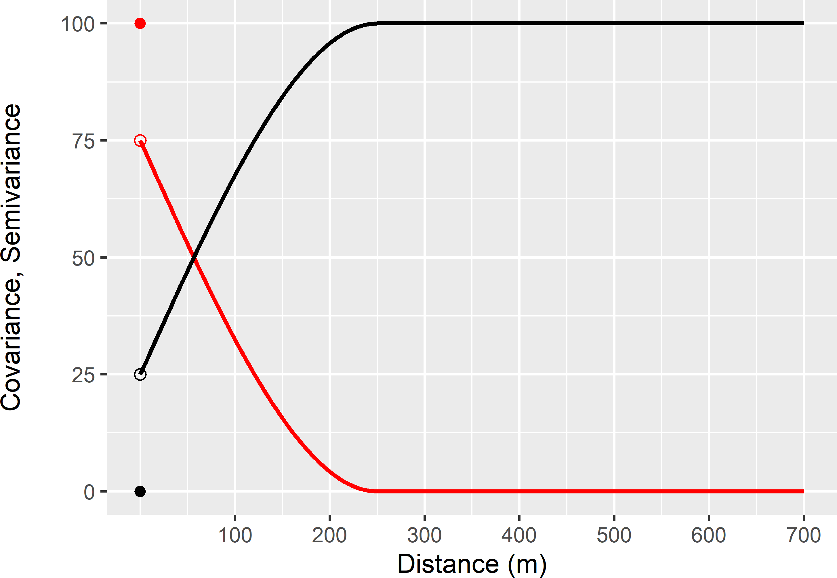
Figure 21.1: Spherical covariance function (red line and dot) and semivariogram (black line and dot).
Expressed in terms of the semivariances between the sampling locations and a prediction location, the OK variance is
\[\begin{equation} V_{\mathrm{OK}}(\widehat{Z}(\mathbf{s}_0))= \lambda^{\mathrm{T}}\pmb{\gamma}_0 + \nu \;, \tag{21.11} \end{equation}\]
with \(\pmb{\gamma}_0\) the vector with semivariances between the sampling locations and a prediction location.
Computing the kriging predictor requires a model for the covariance (or semivariance) as a function of the vector separating two locations. Often, the covariance is modelled as a function of the length of the separation vector only, so as a function of the Euclidian distance between two locations. We then assume isotropy: given a separation distance between two locations, the covariance is the same in all directions. Only authorised functions are allowed for modelling the semivariance, ensuring that the variance of any linear combination of random variables, like the kriging predictor, is positive. Commonly used functions are an exponential and a spherical model.
The spherical semivariogram model has three parameters:
- nugget (\(c_0\)): where the semivariogram touches the y-axis (in Figure 21.1: 25);
- partial sill (\(c_1\)): the difference between the maximum semivariance and the nugget (in Figure 21.1: 75); and
- range (\(\phi\)): the distance at which the semivariance reaches its maximum (in Figure 21.1: 250 m).
The formula for the spherical semivariogram is
\[\begin{equation} \gamma(h)=\left \{ \begin{array}{ll} 0 &\,\,\,\mathrm{if}\,\,\, h=0 \\ c_0+c_1\left[ 1-\frac{3}{2}\left( \frac{h}{\phi}\right) +\frac{1}{2}\left( \frac{h}{\phi}\right) ^{3}\right] &\,\,\,\mathrm{if}\,\,\, 0 < h \leq \phi \\ c_0+c_1 & \,\,\,\mathrm{if}\,\,\, h>\phi \end{array} \right. \;. \tag{21.12} \end{equation}\]
The sum of the nugget and the partial sill is referred to as the sill (or sill variance or a priori variance).
An exponential semivariogram model also has three parameters. Its formula is
\[\begin{equation} \gamma(h)=\left \{ \begin{array}{ll} 0 &\,\,\,\text{if}\,\,\, h=0 \\ c_0+c_1\; \mathrm{exp}(-h/\phi) &\,\,\,\text{if}\,\,\, h > 0 \\ \end{array} \right. \;. \tag{21.13} \end{equation}\]
In an exponential semivariogram, the semivariance goes asymptotically to a maximum; it never reaches it. In an exponential semivariogram, the range parameter is replaced by the distance parameter. In an exponential semivariogram without nugget, the semivariance at three times the distance parameter is at 95% of the sill. Three times the distance parameter is referred to as the effective or practical range.
In following chapters, I also use a correlogram, which is a scaled covariance function, such that the sill of the correlogram equals 1:
\[\begin{equation} \rho(\mathbf{h}) = \frac{C(\mathbf{h})}{\sigma^2} \;. \tag{21.14} \end{equation}\]
To illustrate that the OK variance is independent of the values of the study variable at the sampling locations, I simulated a spatial population of 50 \(\times\) 50 units. For each unit a value of the study variable is simulated, using the semivariogram of Figure 21.1. This is repeated ten times, resulting in ten maps of 2,500 units. Figure 21.2 shows two of the ten simulated maps. Note that the two maps clearly show spatial structure, i.e., there are patches of similar values.
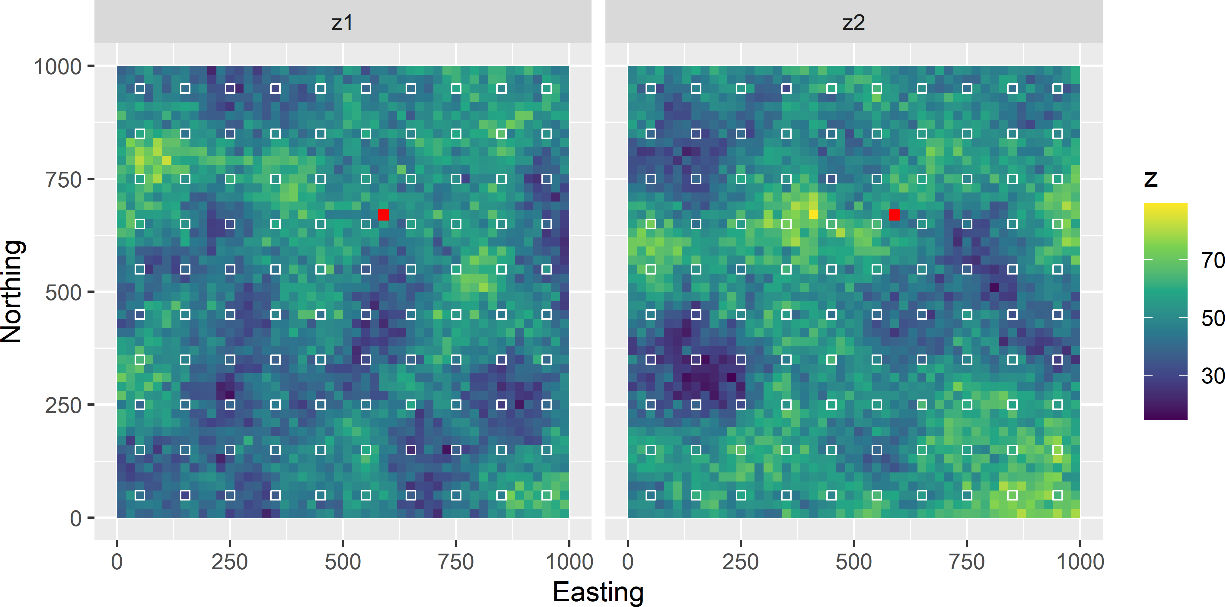
Figure 21.2: Two maps simulated with the spherical semivariogram of Figure 21.1, the centred square grid of sampling units, and the prediction unit (red cell with coordinates (590,670)).
The simulated maps are sampled on a centred square grid with a spacing of 100 distance units, resulting in a sample of 100 units. Each sample is used one-by-one to predict the study variable at one prediction location (see Figure 21.2), using again the semivariogram of Figure 21.1. The semivariogram is passed to function vgm of package gstat (E. J. Pebesma 2004). Usually, this semivariogram is estimated from a sample, see Chapter 24, but here we assume that it is known. Function krige of package gstat is used for kriging. Argument formula specifies the dependent (study variable) and independent variables (covariates). The formula z ~ 1 means that we do not have covariates (we assume that the model-mean is a constant) and that predictions are done by OK (or simple kriging, see Section 21.3). Argument locations is a SpatialPointsDataFrame with the spatial coordinates and observations. Argument newdata is a SpatialPoints object with the locations we want to predict. Argument nmax can be used to specify the neighbourhood in terms of the number of nearest observations to be used in kriging (not used in the code chunk below, so that all 100 observations are used).
library(sp)
library(gstat)
vgmodel <- vgm(model = "Sph", nugget = 25, psill = 75, range = 250)
gridded(mypop) <- ~ s1 + s2
mysample <- spsample(x = mypop, type = "regular", cellsize = c(100, 100),
  offset = c(0.5, 0.5))
zsim_sample <- over(mysample, mypop)
coordinates(s_0) <- ~ s1 + s2
zpred_OK <- v_zpred_OK <- NULL
for (i in seq_len(ncol(zsim_sample))) {
  mysample$z <- zsim_sample[, i]
  predictions <- krige(
    formula = z ~ 1,
    locations = mysample,
    newdata = s_0,
    model = vgmodel,
    debug.level = 0)
  zpred_OK[i] <- predictions$var1.pred
  v_zpred_OK[i] <- predictions$var1.var
}
As can be seen in Table 21.1, unlike the predicted value, the OK variance produced from the different simulations is constant.
| Kriging prediction | Kriging variance |
|---|---|
| 51.44286 | 55.30602 |
| 57.29272 | 55.30602 |
| 52.44407 | 55.30602 |
| 51.40719 | 55.30602 |
| 63.09248 | 55.30602 |
| 40.57517 | 55.30602 |
| 54.48507 | 55.30602 |
| 47.42828 | 55.30602 |
| 43.65313 | 55.30602 |
| 44.52740 | 55.30602 |
21.2 Block-kriging
In the previous section, the support of the prediction units is equal to that of the sampling units. So, if the observations are done at points (point support), the support of the predictions are also points, and if means of small blocks are observed, the predictions are predicted means of blocks of the same size and shape. There is no change of support. In some cases we may prefer predictions at a larger support than that of the observations. For instance, we may prefer predictions of the average concentration of some soil property of blocks of 5 m \(\times\) 5 m, instead of predictions at points, simply because of practical relevance. If the observations are at points, there is a change of support, from points to blocks. Kriging with a prediction support that is larger than the support of the sample data is referred to as block-kriging. Kriging without change of support so that sample support and prediction support are equal, is referred to as point-kriging. Note that point-kriging does not necessarily imply that the support is a point; it can be, for instance, a small block.
In block-kriging the mean of a prediction block \(\mathcal{B}_0\) is predicted as a weighted average of the observations at the sampling units. The kriging weights are derived much in the same way as in point-kriging (Equations (21.4) to (21.7)). In block-kriging the covariance between a sampling point \(i\) and a prediction point, \(C(\mathbf{s}_i,\mathbf{s}_0)\), is replaced by the mean covariance between the sampling point and a prediction block \(\overline{C}(\mathbf{s}_i,\mathcal{B}_0)\) (Equation (21.4)). This mean covariance can be approximated by discretising the prediction block by a fine grid, computing the covariance between a sampling point \(i\) and each of the discretisation points, and averaging.
The variance of the prediction error of the block-mean (block-kriging variance) equals
\[\begin{equation} V_{\mathrm{OBK}}(\widehat{\overline{Z}}(\mathcal{B}_0)) = \lambda^{\mathrm{T}}\bar{\pmb{\gamma}}(\mathcal{B}_0) + \nu - \bar{\gamma}(\mathcal{B}_0,\mathcal{B}_0)\;, \tag{21.15} \end{equation}\]
with \(\bar{\pmb{\gamma}}(\mathcal{B}_0)\) the vector with mean semivariances between the sampling points and a prediction block and \(\bar{\gamma}(\mathcal{B}_0,\mathcal{B}_0)\) the mean semivariance within the prediction block. Comparing this with Equation (21.11) shows that the block-kriging variance is smaller than the point-kriging variance by an amount approximately equal to the mean semivariance within a prediction block. Recall from Chapter 13 that the mean semivariance within a block is a model-based prediction of the variance within a block (Equation (13.3)).
21.3 Kriging with an external drift
In kriging with an external drift (KED), the spatial variation of the study variable is modelled as the sum of a linear combination of covariates and a spatially correlated residual:
\[\begin{equation} \begin{split} Z(\mathbf{s}) & = \sum_{k=0}^p \beta_k x_k(\mathbf{s}) + \epsilon(\mathbf{s}) \\ \epsilon(\mathbf{s}) & \sim \mathcal{N}(0,\sigma^2) \\ \mathrm{Cov}(\epsilon(\mathbf{s}),\epsilon(\mathbf{s}^{\prime})) & = C(\mathbf{h}) \;, \end{split} \tag{21.16} \end{equation}\]
with \(x_k(\mathbf{s})\) the value of the \(k\)th covariate at location \(\mathbf{s}\) (\(x_0\) = 1 for all locations), \(p\) the number of covariates, and \(C(\mathbf{h})\) the covariance of the residuals at two locations separated by vector \(\mathbf{h} = \mathbf{s}-\mathbf{s}^{\prime}\). The constant mean \(\mu\) in Equation (21.2) is replaced by a linear combination of covariates and, as a consequence, the mean is not constant anymore but varies in space.
With KED, the study variable at a prediction location \(\mathbf{s}_0\) is predicted by
\[\begin{equation} \hat{Z}_{\mathrm{KED}}(\mathbf{s}_0)=\sum_{k=0}^p \hat{\beta}_k x_k(\mathbf{s}_0)+\sum_{i=1}^n \lambda_i\left\{Z(\mathbf{s}_i)-\sum_{k=0}^p \hat{\beta}_k x_k(\mathbf{s}_i)\right\}\;, \tag{21.17} \end{equation}\]
with \(\hat{\beta}_k\) the estimated regression coefficient associated with covariate \(x_k\). The first component of this predictor is the estimated model-mean at the new location based on the covariate values at this location and the estimated regression coefficients. The second component is a weighted sum of the residuals at the sampling locations.
The optimal kriging weights \(\lambda_i,\; i = 1, \dots ,n\) are obtained in a similar way as in OK. The difference is that additional constraints on the weights are needed, to ensure unbiased predictions. Not only the weights must sum to 1, but also for all \(p\) covariates the weighted sum of the covariate values at the sampling locations must equal the covariate value at the prediction location: \(\sum_{i=1}^n \lambda_i x_k(\mathbf{s}_i) = x_k(\mathbf{s}_0)\) for all \(k=1, \dots , p\). This leads to a system of \(n+p+1\) simultaneous equations that must be solved. In matrix notation, this system is
\[\begin{eqnarray} \left[ \begin{array}{cc} \mathbf{C} & \mathbf{X} \\ \mathbf{X}^{\mathrm{T}} & \mathbf{0} \\ \end{array} \right] \left[ \begin{array}{c} \pmb{\lambda}\\ \pmb{\nu}\\ \end{array} \right] = \left[ \begin{array}{c} \mathbf{c}_0\\ \mathbf{x}_0\\ \end{array} \right]\;, \tag{21.18} \end{eqnarray}\]
with
\[\begin{eqnarray} \mathbf{X}= \left[ \begin{array}{ccccc} 1&x_{11}&x_{12}&\dots&x_{1p}\\ 1&x_{21}&x_{22}&\dots&x_{2p}\\ \vdots&\vdots&\vdots&\dots&\vdots\\ 1&x_{n1}&x_{n2}&\dots&x_{np}\\ \end{array} \right]\;. \tag{21.19} \end{eqnarray}\]
The submatrix \(\mathbf{0}\) is a \(((p+1) \times (p+1))\) matrix with zeroes, \(\pmb{\nu}\) a (\(p+1\)) vector with Lagrange multipliers, and \(\mathbf{x}_0\) a \((p+1)\) vector with covariate values at the prediction location (including a 1 as the first entry).
The kriging variance with KED equals
\[\begin{equation} V_{\mathrm{KED}}(\widehat{Z}(\mathbf{s}_0))= \sigma^2 - \pmb{\lambda}^{\mathrm{T}}\mathbf{c}_0 - \pmb{\nu}^{\mathrm{T}} \mathbf{x}_0 \;. \tag{21.20} \end{equation}\]
The prediction error variance with KED can also be written as the sum of the variance of the predictor of the mean and the variance of the error in the interpolated residuals (Christensen 1991):
\[\begin{equation} \begin{split} V_{\mathrm{KED}}(\widehat{Z}(\mathbf{s}_0)) &= \sigma^2 - \mathbf{c}_0^{\mathrm{T}}\mathbf{C}^{-1}\mathbf{c}_0 +\\ &(\mathbf{x}_0-\mathbf{X}^{\mathrm{T}}\mathbf{C}^{-1}\mathbf{c}_0)^{\mathrm{T}}(\mathbf{X}^{\mathrm{T}}\mathbf{C}^{-1}\mathbf{X})^{-1}(\mathbf{x}_0-\mathbf{X}^{\mathrm{T}}\mathbf{C}^{-1}\mathbf{c}_0)\;. \end{split} \tag{21.21} \end{equation}\]
The first two terms constitute the interpolation error variance, the third term the variance of the predictor of the mean.
To illustrate that the kriging variance with KED depends on the values of the covariate at the sampling locations and the prediction location, values of a covariate \(x\) and of a correlated study variable \(z\) are simulated for the \(50 \times 50\) units of a spatial population (Figure 21.3). First, a field with covariate values is simulated with a model-mean of 10. Next, a field with residuals is simulated. The field of the study variable is then obtained by multiplying the simulated field with covariate values by two (\(\beta_1=2\)), adding a constant of 10 (\(\beta_0=10\)), and finally adding the simulated field with residuals.
#simulate covariate values
vgm_x <- vgm(model = "Sph", psill = 10, range = 200, nugget = 0)
C <- variogramLine(vgm_x, dist_vector = H, covariance = TRUE)
Upper <- chol(C)
set.seed(314)
N <- rnorm(n = nrow(mypop), 0, 1)
mypop$x <- crossprod(Upper, N) + 10
#simulate values for residuals
vgm_resi <- vgm(model = "Sph", psill = 5, range = 100, nugget = 0)
C <- variogramLine(vgm_resi, dist_vector = H, covariance = TRUE)
Upper <- chol(C)
set.seed(314)
N <- rnorm(n = nrow(mypop), 0, 1)
e <- crossprod(Upper, N)
#compute mean of study variable
betas <- c(10, 2)
mu <- betas[1] + betas[2] * mypop$x
#compute study variable z
mypop$z <- mu  + e
As before, a centred square grid with a spacing of 100 distance units is selected. The simulated values of the study variable \(z\) and covariate \(x\) are used to predict \(z\) at a prediction location \(\mathbf{s}_0\) by kriging with an external drift (red cell in Figure 21.3). Although at the prediction location we have only one simulated value of covariate \(x\), a series of covariate values is used to predict \(z\) at that location: \(x_0 = 0, 2, 4, \dots, 20\). In practice, we have of course only one value of the covariate at a fixed location, but this is for illustration purposes only. Note that we have only one data set with `observations’ of \(x\) and \(z\) at the sampling locations (square grid).
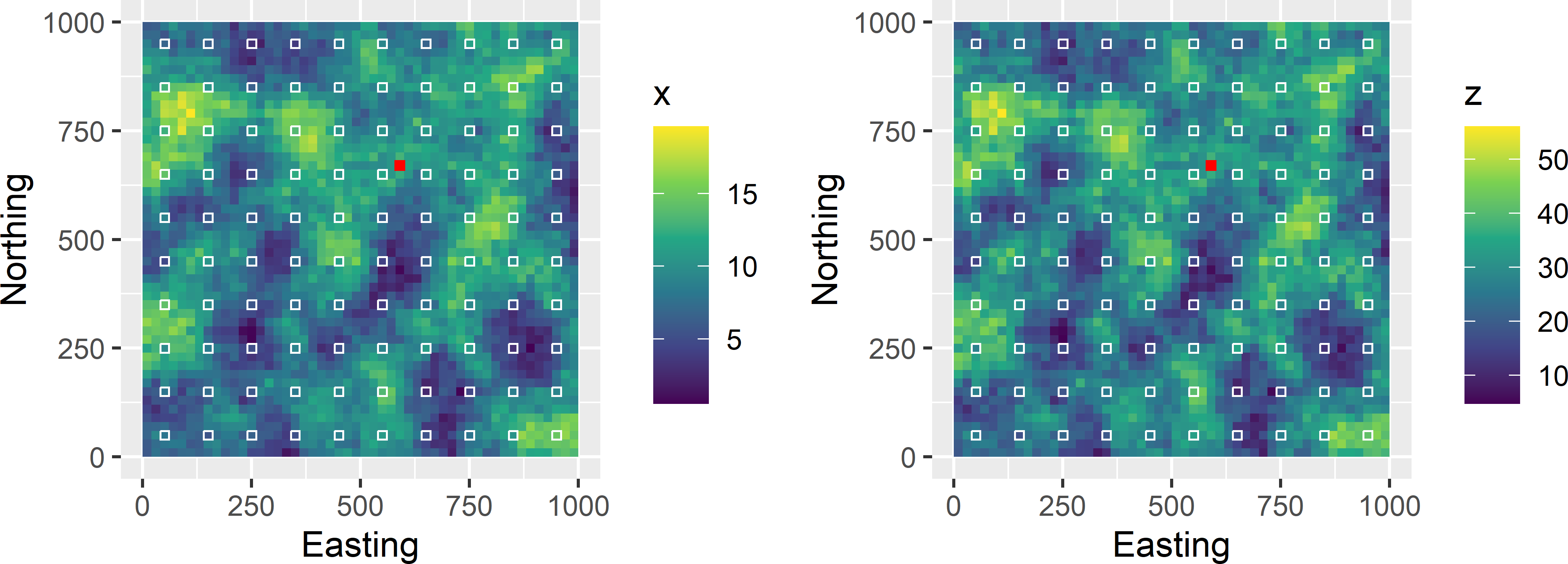
Figure 21.3: Maps with simulated values of covariate \(x\) and study variable \(z\), the centred square grid of sampling units, and the prediction unit (red cell with coordinates (590,670)).
zxsim_sample <- over(mysample, mypop)
mysample$z <- zxsim_sample$z
mysample$x <- zxsim_sample$x
x0 <- seq(from = 0, to = 20, by = 2)
v_zpred_KED <- NULL
for (i in seq_len(length(x0))) {
  s_0$x <- x0[i]
  predictions  <- krige(
    formula = z ~ x,
    locations = mysample,
    newdata = s_0,
    model = vgm_resi,
    debug.level = 0)
  v_zpred_KED[i] <- predictions$var1.var
}
Note the formula z ~ x in the code chunk above, indicating that there is now an independent variable (covariate). The covariate values are attached to the file with the prediction location one-by-one in a for-loop. Also note that for KED we need the semivariogram of the residuals, not of the study variable itself. The residual semivariogram used in prediction is the same as the one used in simulating the fields: a spherical model without nugget, with a sill of 5, and a range of 100 distance units.
To assess the contribution of the uncertainty about the model-mean \(\mu(\mathbf{s})\), I also predict the values assuming that the model-mean is known. In other words, I assume that the two regression coefficients \(\beta_0\) (intercept) and \(\beta_1\) (slope) are known. This type of kriging is referred to as simple kriging (SK). With SK, the constraints explained above are removed, so that there are no Lagrange multipliers involved. Argument beta is used to specify the known regression coefficients. I use the same values used in simulation.
v_zpred_SK <- NULL
for (i in seq_len(length(x0))) {
  s_0$x <- x0[i]
  prediction  <- krige(
    formula = z ~ x,
    locations = mysample,
    newdata = s_0,
    model = vgm_resi,
    beta = betas,
    debug.level = 0)
  v_zpred_SK[i] <- prediction$var1.var
}
Figure 21.4 shows that, contrary to the SK variance, the kriging variance with KED is not constant but depends on the covariate value at the prediction location. It is smallest near the mean of the covariate values at the sampling locations, which is 10.0. The more extreme the covariate value at the prediction location, the larger the kriging variance with KED. This is analogous to the variance of predictions with a linear regression model.
The variance with SK is constant. This is because with SK we assume that the regression coefficients are known, so that we know the model-mean at a prediction location. What remains is the error in the interpolation of the residuals (first two terms in Equation (21.21)). This interpolation error is independent of the value of \(x\) at the prediction location. In Figure 21.4 the difference between the variances with KED and SK is the variance of the predictor of the model-mean, due to uncertainty about the regression coefficients. In real-world applications these regression coefficients are unknown and must be estimated from the sample data. This variance is smallest for a covariate value about equal to the sample mean of the covariate, and increases with the absolute difference of the covariate value and this sample mean.
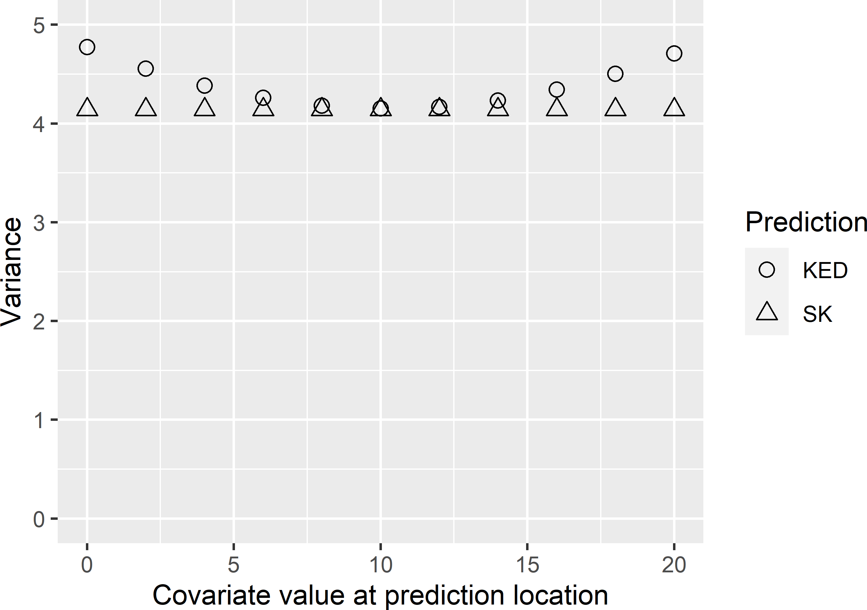
Figure 21.4: Variance of the prediction error as a function of the covariate value at a fixed prediction location, obtained with kriging with an external drift (KED) and simple kriging (SK).
21.4 Estimating the semivariogram
Kriging requires a semivariogram or covariance function as input for computing the covariance matrix of the study variable at the sampling locations, and the vector of covariance of the study variable at the sampling locations and the prediction location. In most cases the semivariogram model is unknown and must be estimated from sample data. The estimated parameters of the semivariogram model are plugged into the kriging equations. There are two different approaches for estimating the semivariogram parameters from sample data: the method-of-moments and maximum likelihood estimation (Lark 2000).
21.4.1 Method-of-moments
With the method-of-moments (MoM) approach, the semivariogram is estimated in two steps. In the first step, a sample semivariogram, also referred to as an experimental semivariogram, is estimated. This is done by choosing a series of distance intervals. If a semivariogram in different directions is required, we must also choose direction intervals.
For each distance interval, all pairs of points with a separation distance in that interval are identified. For each pair, half the squared difference of the study variable is computed, and these differences are averaged over all point-pairs of that interval. This average is the estimated semivariance of that distance interval. The estimated semivariances for all distance intervals are plotted against the average separation distances per distance interval. In the second step, a permissible model is fitted to the sample semivariogram, using some form of weighted least squares. For details, see Webster and Oliver (2007).
The next code chunk shows how this can be done in R. A simple random sample of 150 points is selected from the first simulated field shown in Figure 21.2. Function variogram of package gstat is then used to compute the sample semivariogram. Note that distance intervals need to be passed to function variogram. This can be done with argument width or argument boundaries. In their absence, the default value for argument width is equal to the maximum separation distance divided by 15, so that there are 15 points in the sample semivariogram. The maximum separation distance can be set with argument cutoff. The default value for this argument is equal to one-third of the longest diagonal of the bounding box of the point set. The output is a data frame, with the number of point-pairs, average separation distance, and estimated semivariance in the first three columns.
set.seed(123)
units <- sample(nrow(mypop), size = 150)
mysample <- mypop[units, ]
coordinates(mysample) <- ~ s1 + s2
vg <- variogram(z ~ 1, data = mysample)
head(vg[, c(1, 2, 3)])
np dist gamma
1 35 24.02379 38.73456
2 74 49.02384 42.57199
3 179 78.62401 62.13025
4 213 110.05088 72.41387
5 239 139.20163 82.21432
6 323 170.55712 88.38168The next step is to fit a model. This can be done with function fit.variogram of the gstat package. Many models can be fitted with this function (type vgm() to see all models). I chose a spherical model. Function fit.variogram requires initial values of the semivariogram parameters. From the sample semivariogram, my eyeball estimates are 25 for the nugget, 250 for the range, and 75 for the partial sill. These are passed to function vgm. Figure 21.5 shows the sample semivariogram along with the fitted spherical model11.
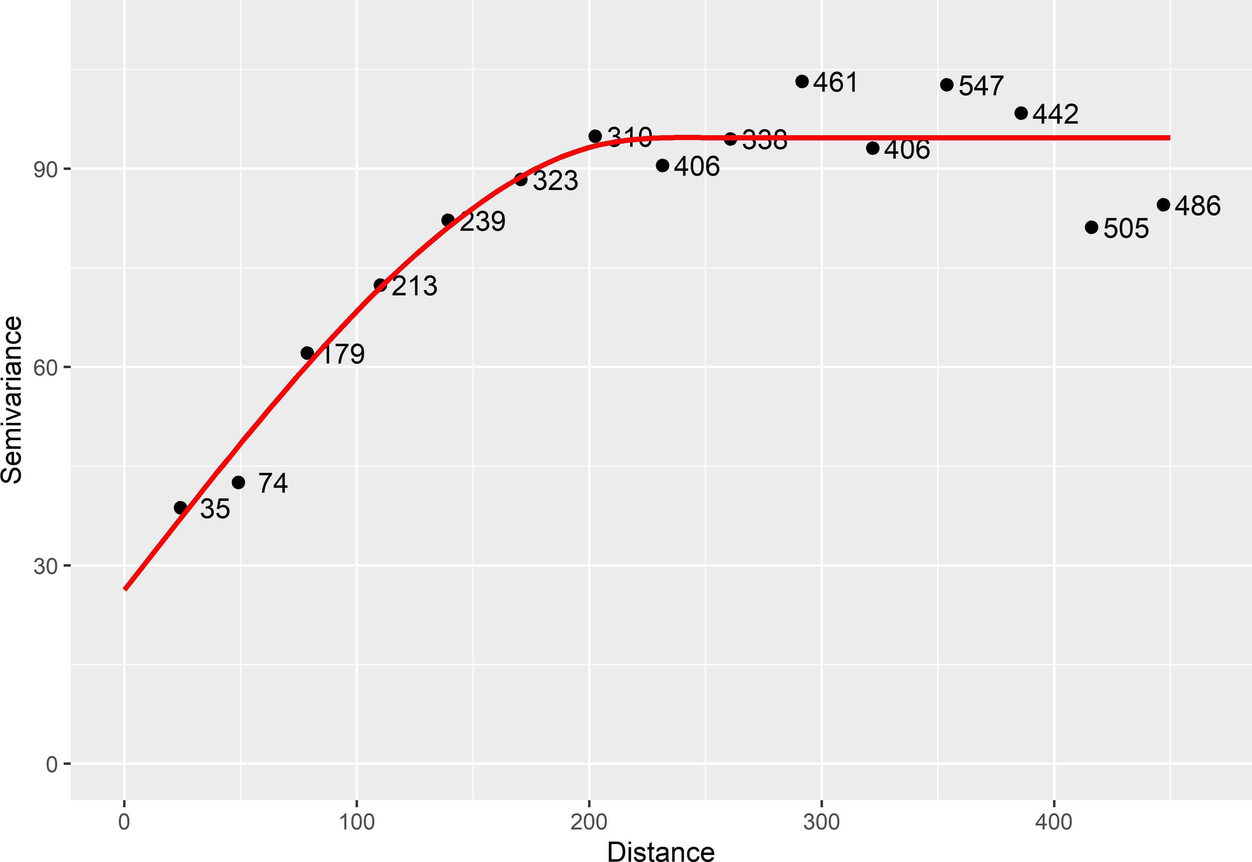
Figure 21.5: Sample semivariogram and fitted spherical model estimated from a simple random sample of 150 units selected from the first simulated field shown in Figure 21.2. Numbers refer to point-pairs used in computing semivariances.
  model    psill    range
1   Nug 26.32048   0.0000
2   Sph 68.36364 227.7999
Function fit.variogram has several options for weighted least squares optimisation, see ?fit.variogram for details. Also note that this non-linear fit may not converge to a solution, especially if the starting values passed to vgm are not near their optimal values.
Further, this method depends on the choice of cutoff and distance intervals. We hope that modifying these does not change the fitted model too much, but this is not always the case, especially with smaller data sets.
21.4.2 Maximum likelihood
In contrast to the MoM, with the maximum likelihood (ML) method the data are not paired into couples and binned into a sample semivariogram. Instead, the semivariogram model is estimated in one step. To apply this method, one typically assumes that (possibly after transformation) the \(n\) sample data come from a multivariate normal distribution. If we have one observation from a normal distribution, the probability density of that observation is given by
\[\begin{equation} f(z|\mu,\sigma ^{2})= \frac{1}{\sigma \sqrt{2\pi }}\exp \left\{ -\frac{1}{2}\left( \frac{z-\mu }{\sigma }\right) ^{2}\right\} \;, \tag{21.22} \end{equation}\]
with \(\mu\) the mean and \(\sigma^2\) the variance. With multiple independent observations, each of them coming from a normal distribution, the joint probability density is given by the product of the probability densities per observation. However, if the data are not independent, we must account for the covariances and the joint probability density can be computed by
\[\begin{equation} f(\mathbf{z}|\pmb{\mu} ,\pmb{\theta})= (2\pi )^{-\frac{n}{2}}|\mathbf{C}|^{-\frac{1}{2}} \exp \left\{ -\frac{1}{2}(\mathbf{z}-\pmb{\mu} )^{\mathrm{T}}\,\mathbf{C}^{-1}\,(\mathbf{z}-\pmb{\mu} )\right\} \;, \tag{21.23} \end{equation}\]
where \(\mathbf{z}\) is the vector with the \(n\) sample data, \(\pmb{\mu}\) is the vector with means, \(\pmb{\theta}\) is the vector with parameters of the covariance function, and \(\mathbf{C}\) is the \(n \times n\) matrix with variances and covariances of the sample data. If the probability density of Equation (21.23) is regarded as a function of \(\pmb{\mu}\) and \(\pmb{\theta}\) with the data \(\mathbf{z}\) fixed, this equation defines the likelihood.
ML estimates of the semivariogram can be obtained with function likfit of package geoR (Ribeiro Jr et al. 2020). First, a geoR object must be made specifying which columns of the data frame contain the spatial coordinates and the study variable.
library(geoR)
mysample <- as(mysample, "data.frame")
dGeoR <- as.geodata(obj = mysample, header = TRUE,
  coords.col = c("s1", "s2"), data.col = "z")
The model parameters can then be estimated with function likfit. Argument trend = "cte" means that we assume that the mean is constant throughout the study area.
vgm_ML <- likfit(geodata = dGeoR, trend = "cte",
  cov.model = "spherical", ini.cov.pars = c(80, 200),
  nugget = 20, lik.method = "ML", messages = FALSE)
Table 21.2 shows the ML estimates together with the MoM estimates. As can be seen, the estimates are substantially different, especially the division of the a priori variance (sill) into partial sill and nugget. In general, I prefer the ML estimates because the arbitrary choice of distance intervals to compute a sample semivariogram is avoided. Also ML estimates of the parameters are more precise, given a sample size. On the other hand, in ML estimation we need to assume that the data are normally distributed.
| Parameter | MoM | ML |
|---|---|---|
| nugget | 26.3 | 19.5 |
| partial sill | 68.4 | 83.8 |
| range | 227.8 | 217.8 |
21.5 Estimating the residual semivariogram
For KED, estimates of the regression coefficients and of the parameters of the residual semivariogram are needed. Estimation of these model parameters is not a trivial problem, as the estimated regression coefficients and the estimated residual semivariogram parameters are not independent. The residuals depend on the estimated regression coefficients and, as a consequence, also the parameters of the residual semivariogram depend on the estimated coefficients. Conversely, the estimated regression coefficients depend on the spatial correlation of the residuals, and so on the estimated residual semivariogram parameters. This is a classic “which came first, the chicken or the egg?” problem.
Estimation of the model parameters is illustrated with the simulated field of Figure 21.3. A simple random sample of size 150 is selected to estimate the model parameters.
21.5.1 Iterative method-of-moments
A simple option is iterative estimation of the regression coefficients followed by MoM estimation of the sample semivariogram and fitting of a semivariogram model. In the first iteration, the regression coefficients are estimated by ordinary least squares (OLS). This implies that the data are assumed independent, i.e., we assume a pure nugget residual semivariogram. The sample semivariogram of the OLS residuals is then computed by the MoM, followed by fitting a model to this sample semivariogram. With package gstat this can be done with one line of R code, using a formula specifying the study variable and the predictors as the first argument of function variogram.
set.seed(314)
units <- sample(nrow(mypop), size = 150)
mysample <- mypop[units, ]
vg_resi <- variogram(z ~ x, data = mysample)
model_eye <- vgm(model = "Sph", psill = 10, range = 150, nugget = 0)
vgmresi_MoM <- fit.variogram(vg_resi, model = model_eye)
Given these estimates of the semivariogram parameters, the regression coefficients are reestimated by accounting for spatial dependency of the residuals. This can be done by generalised least squares (GLS):
\[\begin{equation} \pmb{\hat{\beta}}_{\text{GLS}} = (\mathbf{X}^{\mathrm{T}}\mathbf{C}^{-1}\mathbf{X})^{-1} (\mathbf{X}^{\mathrm{T}}\mathbf{C}^{-1}\mathbf{z})\;. \tag{21.24} \end{equation}\]
The next code chunk shows how the GLS estimates of the regression coefficients can be computed. Function spDists of package sp is used to compute the matrix with distances between the sampling locations, and function variogramLine of package gstat is used to transform the distance matrix into a covariance matrix.
X <- matrix(data = 1, nrow = nrow(as(mysample, "data.frame")), ncol = 2)
X[, 2] <- mysample$x
z <- mysample$z
D <- spDists(mysample)
C <- variogramLine(vgmresi_MoM, dist_vector = D, covariance = TRUE)
Cinv <- solve(C)
XCXinv <- solve(crossprod(X, Cinv) %*% X)
XCz <- crossprod(X, Cinv) %*% z
betaGLS <- XCXinv %*% XCz
The inversion of the covariance matrix \(\mathbf{C}\) can be avoided as follows:
This coding is to be preferred as the inversion of a matrix can be numerically unstable.
The GLS estimates of the regression coefficients can then be used to re-compute the residuals of the mean, and so on, until the changes in the model parameters are negligible.
repeat {
betaGLS.cur <- betaGLS
mu <- X %*% betaGLS
mysample$e <- z - mu
vg_resi <- variogram(e ~ 1, data = mysample)
vgmresi_MoM <- fit.variogram(vg_resi, model = model_eye)
C <- variogramLine(vgmresi_MoM, dist_vector = D, covariance = TRUE)
XCX <- crossprod(X, solve(C, X))
XCz <- crossprod(X, solve(C, z))
betaGLS <- solve(XCX, XCz)
if (sum(abs(betaGLS - betaGLS.cur)) < 0.0001) {
break
}
}Table 21.3 shows the estimates of the residual semivariogram parameters and regression coefficients, together with the estimates obtained by restricted maximum likelihood, which is explained in the next subsection.
21.5.2 Restricted maximum likelihood
The estimates of the residual semivariogram parameters obtained by the iterative MoM procedure are not unbiased. When the mean is not constant but is a linear combination of one or more covariates, also ML estimation results in biased estimates of the residual semivariogram parameters. Unbiased estimates of the regression coefficients and residual semivariogram parameters can be obtained by restricted maximum likelihood (REML), also referred to as residual maximum likelihood. In REML the vector with the data is premultiplied by a so-called projection matrix \(\mathbf{P}\) (Kitanidis 1983). This projection matrix has the property that a vector with zeroes is obtained when the matrix \(\mathbf{X}\) with the covariate values at the sampling locations (and ones in the first column) is premultiplied with \(\mathbf{P}\):
\[\begin{equation} \mathbf{P}\mathbf{X}=\mathbf{0} \;. \tag{21.25} \end{equation}\]
Premultiplying both sides of the KED model (Equation (21.16)) with \(\mathbf{P}\) gives (Webster and Oliver 2007)
\[\begin{equation} \mathbf{P}\mathbf{z}(\mathbf{s})=\mathbf{y}(\mathbf{s})=\mathbf{P}\mathbf{X}\pmb{\beta} + \mathbf{P}\pmb{\epsilon}(\mathbf{s})=\mathbf{P}\pmb{\epsilon}(\mathbf{s}) \;. \tag{21.26} \end{equation}\]
In words, by premultiplying variable \(\mathbf{z}\) with matrix \(\mathbf{P}\), a new variable \(\mathbf{y}\) is obtained that has a constant mean. So, the trend is filtered out, whatever the regression coefficients are. The semivariogram parameters of this new variable can be estimated by ML. The projection matrix \(\mathbf{P}\) can be computed by
\[\begin{equation} \mathbf{P}=\mathbf{I}-\mathbf{X}(\mathbf{X}^{\mathrm{T}}\mathbf{X})^{-1}\mathbf{X}^{\mathrm{T}} \;, \tag{21.27} \end{equation}\]
with \(\mathbf{I}\) the \(n \times n\) identity matrix (matrix with ones on the diagonal and zeroes in all off-diagonal elements). The natural log of the residual likelihood can be computed by (Lark and Webster 2006)
\[\begin{equation} \ell(\pmb{\theta}|\mathbf{z})=\mathrm{constant}-0.5(\mathrm{ln}|\mathbf{C}|+|\mathbf{X}^{\mathrm{T}}\mathbf{C}^{-1}\mathbf{X}|+\mathbf{y}^{\mathbf{T}}\mathbf{C}^{-1}(\mathbf{I-\mathbf{Q}})\mathbf{z})) \;, \tag{21.28} \end{equation}\]
with \(\mathbf{Q} = \mathbf{X}(\mathbf{X}^{\mathrm{T}}\mathbf{C}^{-1}\mathbf{X})^{-1}\mathbf{X}^{\mathrm{T}}\mathbf{C}^{-1}\)
REML estimates of the semivariogram can be obtained with function likfit of package geoR, used above in ML estimation of the variogram (Ribeiro Jr et al. 2020).
vgm_REML <- likfit(geodata = dGeoR, trend = ~ x,
  cov.model = "spherical", ini.cov.pars = c(2, 100),
nugget = 0, lik.method = "REML", messages = FALSE)| Parameter | iMoM | REML |
|---|---|---|
| nugget | 0.000 | 0.000 |
| partial sill | 2.137 | 1.909 |
| range | 129.147 | 141.491 |
| intercept | 3.255 | 3.083 |
| x | 2.712 | 2.732 |
Table 21.3 shows that REML yields a smaller estimated (partial) sill and a larger estimated range than iterative MoM. Of the two regression coefficients, especially the estimated intercept differs considerably among the two estimation methods.
Realising that this is a rather short introduction to kriging, refer to Isaaks and Srivastava (1989) for an introduction to geostatistics, to Goovaerts (1997) for an expos\(\acute{\text{e}}\) of the many versions of kriging, and to Webster and Oliver (2007) for an elaborate explanation of kriging. A nice educational tool for getting a feeling for ordinary kriging is E{Z}-Kriging.