Chapter 11 Two-phase random sampling
The regression and ratio estimators of Chapter 10 require that the means of the ancillary variables are known. If these are unknown, but the ancillary variables can be measured cheaply, one may decide to estimate the population means of the ancillary variables from a large sample. The study variable is measured in a random subsample of this large sample only. This technique is known in the sampling literature as two-phase random sampling or double sampling. Another application of two-phase sampling is two-phase sampling for stratification. Stratified random sampling (Chapter 4) requires a map with the strata. The poststratified estimator of Subsection 10.3 requires that the sizes of the strata are known. With two-phase sampling for stratification, neither a map of the strata nor knowledge of the stratum sizes is required. Note that the term `phase’ does not refer to a period of time; all data can be collected in one sampling campaign. Let me also explain the difference with two-stage cluster sampling (Chapter 7). In two-stage cluster random sampling, we have two types of sampling units, clusters of population units and individual population units. In two-phase sampling, we have one type of sampling unit only, the objects of a discrete population or the elementary sampling units of a continuous population (Section 1.1).
In two-phase sampling for regression and two-phase sampling for stratification, the two phases have the same aim, i.e., to estimate the population mean of the study variable. The observations of the covariate(s) and/or strata in the first phase are merely done to increase the precision of the estimated mean of the study variable. Another application of two-phase sampling is subsampling an existing probability sample designed for a different aim. So, in this case the study variable observed in the second-phase sample may not be related to the variables observed in the first-phase sample.
An example is LUCAS-Topsoil (Ballabio et al. 2019) which is a subsample of approximately 22,000 units sampled from a much larger sample, the LUCAS sample, designed for estimating totals of land use and land cover classes across the European Union. It was not feasible to observe the soil properties at all sites of the LUCAS sample, and for this reason a subsample was selected. Regrettably, this subsample is not a probability sample from the LUCAS sample: the inclusion probabilities are either zero or unknown. Design-based or model-assisted estimation of means of soil properties for domains of interest is not feasible. The only option is model-based prediction.
In case the subsample is a probability subsample from the first-phase sample and no variable observed in the first-phase sample is of use for estimating the total or mean of the study variable observed in the subsample, the population total can be estimated by the \(\pi\) estimator:
\[\begin{equation} \hat{t}(z) =\sum_{k \in \mathcal{S}_2}\frac{z_k}{\pi_{1k}\pi_{k|\mathcal{S}_1}} =\sum_{k \in \mathcal{S}_2}\frac{z_k}{\pi^*_{k}} \;, \tag{11.1} \end{equation}\]
with \(\pi_{1k}\) the probability that unit \(k\) is selected in the first phase, and \(\pi_{k|\mathcal{S}_1}\) the probability that unit \(k\) is selected in the second phase, given the first-phase sample \(\mathcal{S}_1\). This general \(\pi\) estimator for two-phase sampling, referred to as the \(\pi^*\) estimator by Särndal, Swensson, and Wretman (1992), can be used for any combination of probability sampling designs in the first and second phase.
To derive the variance, it is convenient to write the total estimation error as the sum of two errors:
\[\begin{equation} \begin{split} \hat{t}(z)-t(z) &=\left(\sum_{k \in \mathcal{S}_1}\frac{z_k}{\pi_{1k}}-t(z)\right)+\left(\sum_{k \in \mathcal{S}_2}\frac{z_k}{\pi^*_{k}}-\sum_{k \in \mathcal{S}_1}\frac{z_k}{\pi_{1k}}\right)\\ & =e_1+e_2 \;. \end{split} \tag{11.2} \end{equation}\]
The first error \(e_1\) is the error in the estimated population total, as estimated by the usual \(\pi\) estimator using the study variable values for the units in the first-phase sample. This estimator cannot be computed in practice, as the study variable values are only known for a subset of the units in the first-phase sample. The second error \(e_2\) is the difference between the \(\pi^*\) estimator using the study variable values for the units in the subsample only, and the \(\pi\) estimator using the study variable values for all units in the first-phase sample.
The variance of the \(\pi^*\) estimator can be decomposed into the variance of these two errors as follows:
\[\begin{equation} V_{p_1,p_2}(\hat{t})=V_{p_1}E_{p_2}(\hat{t}|\mathcal{S}_1)+E_{p_1}V_{p_2}(\hat{t}|\mathcal{S}_1)=V_{p_1}(e_1)+E_{p_1}V_{p_2}(e_2|\mathcal{S}_1)\;, \tag{11.3} \end{equation}\]
with \(V_{p_1}\) and \(E_{p_1}\) the variance and expectation of the estimator for the population total over repeated sampling with the design of the first phase, respectively, and \(V_{p_2}\) and \(E_{p_2}\) the variance and expectation of the estimator for the population total over repeated sampling with the design of the second phase, respectively. The population mean can be estimated by the estimated total divided by the population size \(N\).
11.1 Two-phase random sampling for stratification
In two-phase sampling for stratification, in the first phase a large sample is taken and the selected sampling units are all classified. The classes thus formed are then used as strata in the second sampling phase. A stratified subsample is selected, and the study variable is observed on the units in the subsample only.
Two-phase sampling for stratification is now illustrated with study area Voorst. A map with five combinations of soil type and land use is available of this study area. These combinations were used as strata in Chapter 4, and the stratum sizes were used in the poststratified estimator of Subsection 10.3. Here, we consider the situation that we do not have this map and that we do not know the sizes of these strata either. In the first phase, a simple random sample of size 100 is selected. In the field, the soil-land use combination is determined for the selected points, see Figure 11.1. This time we assume that the field determinations are equal to the classes as shown on the map.
n1 <- 100
set.seed(123)
N <- nrow(grdVoorst)
units <- sample(N, size = n1, replace = FALSE)
mysample <- grdVoorst[units, ]
The simple random sample is subsampled by stratified simple random sampling, using the soil-land use classes as strata. The total sample size of the second phase is set to 40. The number of points in the simple random sample per stratum is determined. Then the subsample size per stratum is computed for proportional allocation. Finally, function strata of package sampling (Tillé and Matei 2021) is used to select a stratified simple random sample without replacement, see Chapter 4 for details. At the 40 points of the second-phase, the soil organic matter (SOM) concentration is measured.
library(sampling)
n2 <- 40
n1_h <- tapply(mysample$z, INDEX = mysample$stratum, FUN = length)
n2_h <- round(n1_h / n1 * n2, 0)
units <- sampling::strata(mysample, stratanames = "stratum",
  size = n2_h[unique(mysample$stratum)], method = "srswor")
mysubsample <- getdata(mysample, units)
table(mysubsample$stratum)
BA EA PA RA XF
15 8 6 4 7 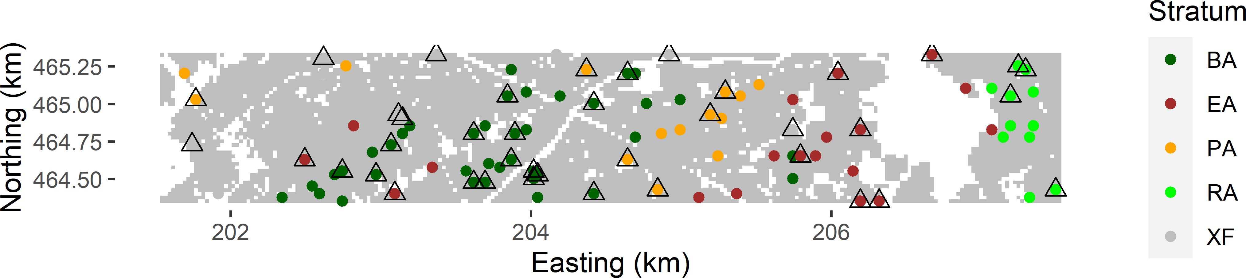
Figure 11.1: Two-phase random sample for stratification from Voorst. Coloured dots: first-phase sample of 100 points selected by simple random sampling, with observations of the soil-land use combination. Triangles: second-phase sample of 40 points selected by stratified simple random subsampling of the first-phase sample, using the soil-land use combinations as strata, with measurements of SOM.
With simple random sampling in the first phase and stratified simple random sampling in the second phase, the population mean can be estimated by
\[\begin{equation} \hat{\bar{z}}= \sum_{h=1}^{H_{\mathcal{S}_1}}\frac{n_{1h}}{n_{1}}\,\bar{z}_{\mathcal{S}_{2h}} \;, \tag{11.4} \end{equation}\]
where \(H_{\mathcal{S}_1}\) is the number of strata used for stratification of the first-phase sample, \(n_{1h}\) is the number of units in the first-phase sample that form stratum \(h\) in the second phase, \(n_{1}\) is the total number of units of the first-phase sample, and \(\bar{z}_{\mathcal{S}_{2h}}\) is the mean of the subsample from stratum \(h\).
mz_h_subsam <- tapply(mysubsample$z, INDEX = mysubsample$stratum, FUN = mean)
mz <- sum(n1_h / n1 * mz_h_subsam, na.rm = TRUE)
The estimated population mean equals 85.6 g kg-1. The sampling variance over repeated sampling with both designs can be approximated5 by (Särndal, Swensson, and Wretman (1992), equation at bottom of p. 353)
\[\begin{equation} \widehat{V}\!(\hat{\bar{z}}) = \sum_{h=1}^{H_{\mathcal{S}_1}}\left( \frac{n_{1h}}{n_1}\right)^2 \frac{\widehat{S^2}_{\mathcal{S}_{2h}}}{n_{2h}} + \frac{1}{n_1}\sum_{h=1}^{H_{\mathcal{S}_1}} \frac{n_{1h}}{n_1}\left( \bar{z}_{\mathcal{S}_{2h}}-\hat{\bar{z}}\right)^2 \;, \tag{11.5} \end{equation}\]
with \(\widehat{S^2}_{\mathcal{S}_{2h}}\) the variance of \(z\) in the subsample from stratum \(h\).
S2z_h_subsam <- tapply(mysubsample$z, INDEX = mysubsample$stratum, FUN = var)
w1_h <- n1_h / n1
v_mz_1 <- sum(w1_h^2 * S2z_h_subsam / n2_h)
v_mz_2 <- 1 / n1 * sum(w1_h * (mz_h_subsam - mz)^2)
se_mz <- sqrt(v_mz_1 + v_mz_2)
The estimated standard error equals 7.1 g kg-1.
The mean and its standard error can be estimated with functions twophase and svymean of package survey (Lumley 2021). A data frame with the first-phase sample is passed to function twophase using argument data. A variable in this data frame, passed to function twophase with argument subset, is an indicator with value TRUE if this unit is selected in the second phase, and FALSE otherwise.
library(survey)
lut <- data.frame(stratum = sort(unique(mysample$stratum)), fpc2 = n1_h)
mysample <- mysample %>%
  mutate(ind = FALSE,
         fpc1 = N) %>%
  left_join(lut, by = "stratum")
mysample$ind[units$ID_unit] <- TRUE
design_2phase <- survey::twophase(
  id = list(~ 1, ~ 1), strata = list(NULL, ~ stratum),
  data = mysample, subset = ~ ind, fpc = list(~ fpc1, ~ fpc2))
svymean(~ z, design_2phase)
mean SE
z 85.606 7.033As shown in the next code chunk, the standard error is computed with the original variance estimator, without approximation (Särndal, Swensson, and Wretman (1992), equation (9.4.14)).
v_mz_1 <- 1 / N^2 * N * (N - 1) *
  sum((((n1_h - 1) / (n1 - 1)) - ((n2_h - 1) / (N - 1)))
      * w1_h * S2z_h_subsam / n2_h)
v_mz_2 <- 1 / N^2 * (N * (N - n1)) / (n1 - 1) *
  sum(w1_h * (mz_h_subsam - mz)^2)
sqrt(v_mz_1 + v_mz_2)
[1] 7.03296411.2 Two-phase random sampling for regression
The simple regression estimator of Equation (10.10) requires that the population mean of the ancillary variable \(x\) is known. This section, however, is about applying the regression estimator in situations where the mean of \(x\) is unknown. A possible application is estimating the soil organic carbon (SOC) stock in an area. To estimate this carbon stock, soil samples are collected and analysed in a laboratory. The laboratory measurements can be very accurate, but also expensive. Proximal sensors can be used to derive soil carbon concentrations from the spectra. Compared to laboratory measurements of soil the proximal sensor determinations are much cheaper, but also less accurate. If there is a relation between the laboratory and the proximal sensing determinations of SOC, then we expect that the regression estimator of the carbon stock will be more accurate than the \(\pi\) estimator which does not exploit the proximal sensing measurements. However, the population mean of the proximal sensing determinations is unknown. What we can do is estimate this mean from a large sample. Additionally, for a subsample of this large sample, SOC concentration is also measured in the laboratory. This is another example of two-phase sampling.
Intuitively, we understand that with two-phase sampling the variance of the regression estimator of the total carbon stock is larger than when the population mean of the proximal sensing determinations is known. There is a sampling error in the estimated population mean of the proximal sensing determinations, estimated from the large first-phase sample, and this error propagates to the error in the estimated total carbon stock.
Two-phase sampling for regression is now illustrated with Eastern Amazonia (Subsection 1.3.3). The study variable is the aboveground biomass (AGB), and lnSWIR2 is used here as a covariate. We do have a full coverage map of lnSWIR2, so two-phase sampling with a large first-phase sample to estimate the population mean of lnSWIR2 is not needed. Nevertheless, hereafter a two-phase sample is selected, and the population mean of lnSWIR2 is estimated from the first-phase sample. In doing so, the effect of ignorance of the population mean of the covariate on the variance of the regression estimator becomes apparent.
In the next code chunk, a first-phase sample of 250 units, the dots in the plot, is selected by simple random sampling without replacement. In the second phase a subsample of 100 units, the triangles in the plot, is selected from the 250 units by simple random sampling without replacement. At all 250 units of the first-phase sample the covariate lnSWIR2 is measured, whereas AGB is measured at the 100 subsample units only.
grdAmazonia <- grdAmazonia %>%
  mutate(lnSWIR2 = log(SWIR2))
n1 <- 250; n2 <- 100
set.seed(314)
units_1 <- sample(nrow(grdAmazonia), size = n1, replace = FALSE)
mysample <- grdAmazonia[units_1, ]
units_2 <- sample(n1, size = n2, replace = FALSE)
mysubsample <- mysample[units_2, ]
Figure 11.2 shows the selected two-phase sample.
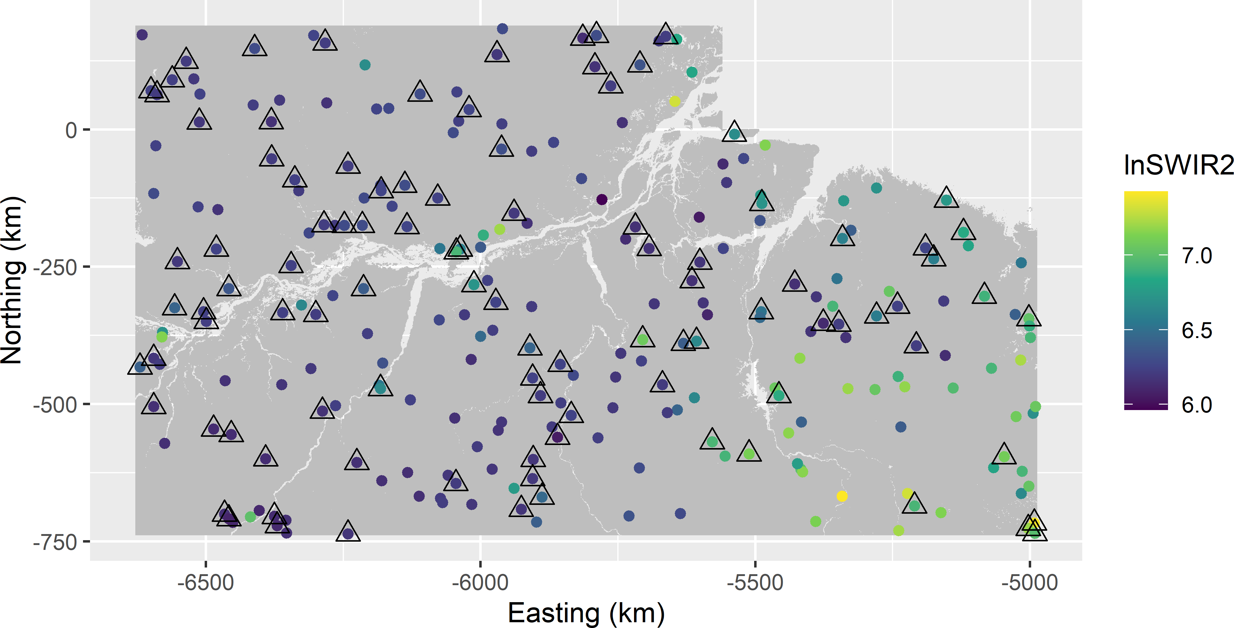
Figure 11.2: Two-phase random sample for the regression estimator of the mean AGB in Eastern Amazonia. Coloured dots: simple random sample without replacement of 250 units with measurements of covariate lnSWIR2 (first-phase sample). Triangles: simple random subsample without replacement of 100 units with measurements of AGB (second-phase sample).
Estimation of the population mean or total by the regression estimator from a two-phase sample is very similar to estimation when the covariate mean is known, as described in Subsection 10.1.1 (Equation (10.10)). The observations of the subsample can be used to estimate the regression coefficient \(b\). The true population mean of the ancillary variable, \(\bar{x}\) in Equation (10.10), is unknown now. This true mean is replaced by the mean as estimated from the relatively large first-phase sample, \(\bar{x}_{\mathcal{S}_1}\). The estimated mean of the covariate, \(\bar{x}_{\mathcal{S}}\) in Equation (10.10), is estimated from the subsample, \(\bar{x}_{\mathcal{S}_2}\). This leads to the following estimator:
\[\begin{equation} \hat{\bar{z}}= \bar{z}_{\mathcal{S}_2}+\hat{b}\left( \bar{x}_{\mathcal{S}_1}-\bar{x}_{\mathcal{S}_2}\right) \;, \tag{11.6} \end{equation}\]
where \(\bar{z}_{\mathcal{S}_2}\) is the subsample mean of the study variable, and \(\bar{x}_{\mathcal{S}_1}\) and \(\bar{x}_{\mathcal{S}_2}\) are the means of the covariate in the first-phase sample and the subsample (i.e., the second-phase sample), respectively.
The sampling variance is larger than that of the regression estimator with known mean of \(x\). The variance can be decomposed into two components. The first component is equal to the sampling variance of the \(\pi\) estimator of the mean of \(z\) with the sampling design of the first phase (in this case, simple random sampling without replacement), supposing that the study variable is observed on all units of the first-phase sample. The second component is equal to the sampling variance of the regression estimator of the mean of \(z\) in the first-phase sample, with the design of the second-phase sample (again simple random sampling without replacement in this case):
\[\begin{equation} \widehat{V}\!\left(\hat{\bar{z}}\right)=(1-\frac{n_1}{N})\frac{\widehat{S^{2}}(z)}{n_1} + (1-\frac{n_2}{n_1}) \frac{\widehat{S^{2}}(e)}{n_2} \;, \tag{11.7} \end{equation}\]
with \(\widehat{S^{2}}(e)\) the variance of the regression residuals as estimated from the subsample:
\[\begin{equation} \widehat{S^{2}}(e)=\frac{1}{(n_2-1)}\sum_{k \in \mathcal{S}_2}e_{k}^2 \;. \tag{11.8} \end{equation}\]
The ratios \((1-n_1/N)\) and \((1-n_2/n_1)\) in Equation (11.7) are finite population corrections (fpcs). These fpcs account for the reduced variance due to sampling the finite population and subsampling the first-phase sample without replacement.
lm_subsample <- lm(AGB ~ lnSWIR2, data = mysubsample)
ab <- coef(lm_subsample)
mx_sam <- mean(mysample$lnSWIR2)
mx_subsam <- mean(mysubsample$lnSWIR2)
mz_subsam <- mean(mysubsample$AGB)
mz_reg2ph <- mz_subsam + ab[2] * (mx_sam - mx_subsam)
The estimated population mean equals 228.1 109 kg ha-1. The standard error can be approximated as follows.
e <- residuals(lm_subsample)
S2e <- sum(e^2) / (n2 - 1)
S2z <- var(mysubsample$AGB)
N <- nrow(grdAmazonia)
se_mz_reg2ph <- sqrt((1 - n1 / N) * S2z / n1 + (1 - n2 / n1) * S2e / n2)
The estimated standard error equals 6.35 109 kg ha-1.
The regression estimator for two-phase sampling and its standard error can also be computed with package survey, as shown below. The standard error differs from the standard error computed above because it is computed with the g-weights, see Subsection 10.1.1. Note argument fpc = list(~ N, NULL). There is no need to add the first-phase sample size as a second element of the list, because this sample size is simply the number of rows of the data frame. Setting the second element of the list to NULL does not mean that the standard error is computed for sampling with replacement in the second phase. Function twophase assumes that the second-phase units are always selected without replacement.
mysample <- mysample %>%
  mutate(id = row_number(),
         N = N,
         ind = id %in% units_2)
design_2phase <- survey::twophase(
  id = list(~ 1, ~ 1), data = mysample, subset = ~ ind, fpc = list(~ N, NULL))
mysample_cal <- calibrate(
  design_2phase, formula = ~ lnSWIR2, calfun = "linear", phase = 2)
svymean(~ AGB, mysample_cal)
mean SE
AGB 228.07 7.2638Exercises
- Write an R script to select a simple random sample without replacement of 250 units from Eastern Amazonia and a subsample of 100 units by simple random sampling without replacement. Repeat this 1,000 times in a for-loop.
- Use each sample selected in the first phase (sample of 250 units) to estimate the population mean of AGB by the regression estimator (Equation (10.10) in Chapter 10). Assume that the AGB data are known for all units selected in the first phase. Use lnSWIR2 as a covariate.
- Compute the variance of the 10,000 regression estimates of the population mean of AGB.
- Use each two-phase sample to compute the regression estimator of AGB for two-phase sampling (Equation (11.6)). Now only use the AGB data of the subsample. Estimate the population mean of lnSWIR2 from the first-phase sample of 250 units. Approximate the variance of the regression estimator for two-phase sampling (Equation (11.7)).
- Compute the variance of the 10,000 regression estimates of the population mean of AGB for the two-phase sampling design.
- Compare the two variances and explain the difference.
- Compute the average of the 10,000 approximate variances and compare the result with the variance of the 10,000 estimated means, as estimated by the regression estimator for two-phase sampling.
References
In the approximation, it is assumed that \(N\) is much larger than \(n_1\), and \((n_{1h}-1)/(n_1-1)\) is replaced by \(n_{1h}/n_1\).↩︎