Chapter 26 Design-based, model-based, and model-assisted approach for sampling and inference
Section 1.2 already mentioned the design-based and the model-based approach for sampling and statistical inference. In this chapter, the fundamental differences between these two approaches are explained in more detail. Several misconceptions about the design-based approach for sampling and statistical inference, based on classical sampling theory, seem to be quite persistent. These misconceptions are the result of confusion about basic statistical concepts such as independence, expectation, and bias and variance of estimators or predictors. These concepts have a different meaning in the design-based and the model-based approach. Besides, a population mean is still often confused with a model-mean, and a population variance with a model-variance, leading to invalid formulas for the sampling variance of an estimator of the population mean. The fundamental differences between these two approaches are illustrated with simulations, so that hopefully a better understanding of this subject is obtained. Besides, the difference between model-dependent inference (as used in the model-based approach) and model-assisted inference is explained. This chapter has been published as part of a journal paper, see Brus (2021).
26.1 Two sources of randomness
In my classes about spatial sampling, I ask the participants the following question. Suppose we have measurements of a soil property, for instance soil organic carbon content, at two locations separated by 20 cm. Do you think these two measurements are correlated? I ask them to vote for one of three answers:
- yes, they are (>80% confident);
- no, they are not (>80% confident); or
- I do not know.
Most students vote for answer 1, the other students vote for answer 3, nearly no one votes for answer 2. Then I explain that you cannot say which answer is correct, simply because for correlation we need two series of data, not just two numbers. The question then is how to generate two series of data. We need some random process for this. This random process differs between the design-based and the model-based approach.
In the design-based approach, the random process is the random selection of sampling units, whereas in the model-based approach randomness is introduced via the statistical model of the spatial variation (Table 1.1). So, the design-based approach requires probability sampling, i.e., random sampling, using a random number generator, in such way that all population units have a positive probability of being included in the sample and that these inclusion probabilities are known for at least the selected population units (Särndal, Swensson, and Wretman 1992). A probability sampling design can be used to generate an infinite number of samples in theory, although in practical applications only one is selected.
The spatial variation model used in the model-based approach contains two terms, one for the mean (deterministic part) and one for the error with a specified probability distribution. For instance, Equation (21.2) in Chapter 21 describes the model used in ordinary kriging. This model can be used to simulate an infinite number of spatial populations. All these populations together are referred to as a superpopulation (Särndal, Swensson, and Wretman (1992), Lohr (1999)). Depending on the model of spatial variation, the simulated populations may show spatial structure because the mean is a function of covariates, as in kriging with an external drift, and/or because the errors are spatially autocorrelated. A superpopulation is a construct, the populations do not exist in the real world. The populations are similar, but not identical. For instance, the mean differs among the populations. The expectation of the population mean, i.e., the average over all possible simulated populations, equals the superpopulation mean, commonly referred to as the model-mean, parameter \(\mu\) in Equation (21.2). The variance also differs among the populations. Contrary to the mean, the average of the population variance over all populations generally is not equal to the model-variance, parameter \(\sigma^2\) in Equation (21.2), but smaller. I will come back to this later. The differences between the simulated spatial populations illustrate our uncertainty about the spatial variation of the study variable in the population that is sampled or will be sampled.
In the design-based approach, only one population is considered, the one sampled, but the statistical inference is based on all samples that can be generated by a probability sampling. The top row of Figure 26.1 shows five simple random samples of size ten. The population is the same in all plots. Proponents of the design-based approach do not like to consider other populations than the one sampled. Their challenge is to characterise this one population from a probability sample.
On the contrary, in the model-based approach only one sample is considered, but the statistical inference is based on all populations that can be generated with the spatial variation model. Proponents of the model-based approach do not like to consider other samples than the one selected. Their challenge is to get the most out of the sample that is selected. The bottom row of Figure 26.1 shows a spatial coverage sample, superimposed on five different populations simulated with an ordinary kriging model, using a spherical semivariogram with a nugget of 0.1, partial sill of 0.6, and a range of 75 m. Note that in the model-based approach there is no need to select a probability sample (see Table 1.1); there are no requirements on how the units are selected.
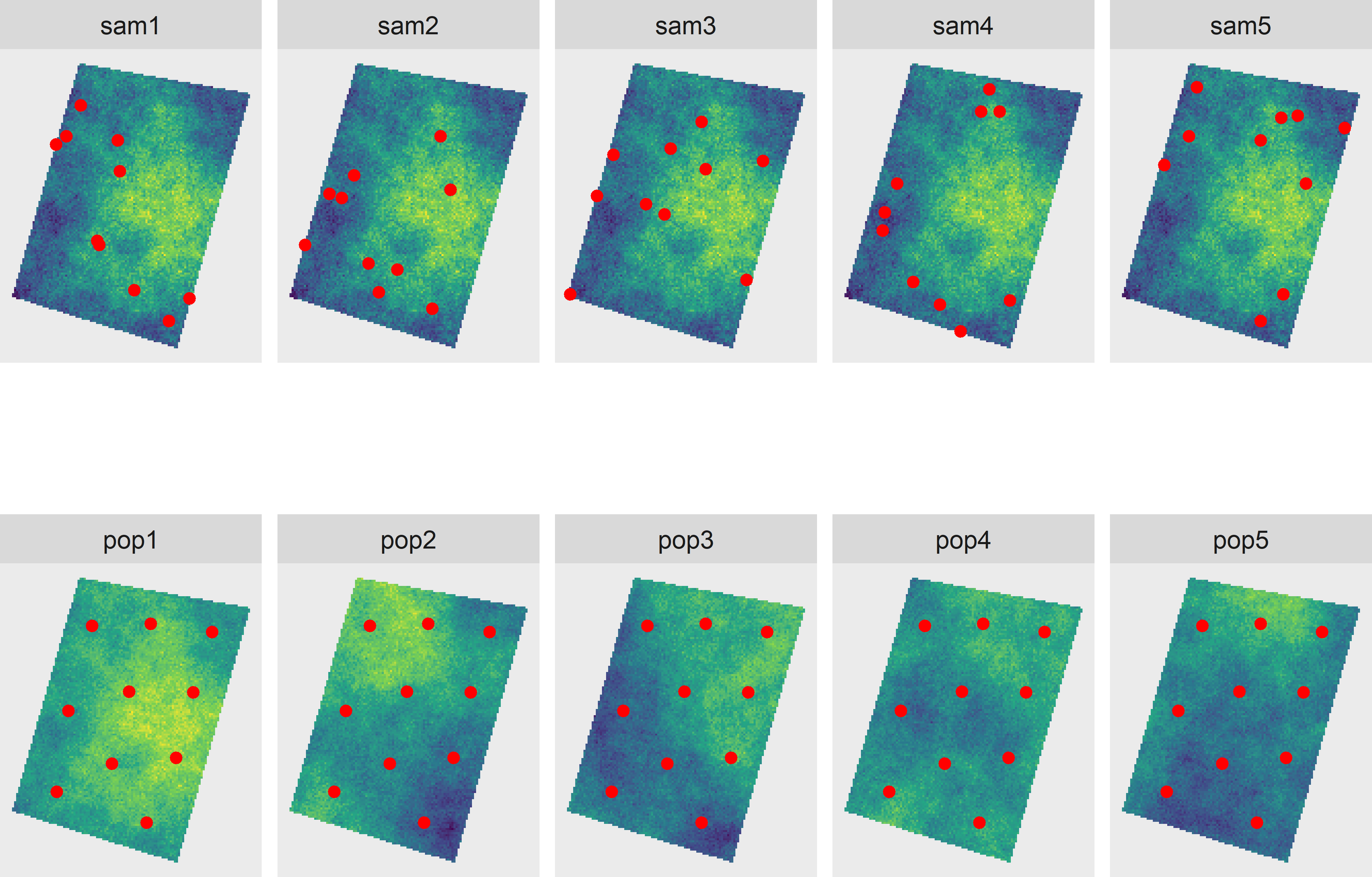
Figure 26.1: Random process considered in the design-based (top row) and the model-based approach (bottom row). The design-based approach considers only the sampled population, but all samples that can be generated by the sampling design. The model-based approach considers only the selected sample, but all populations that can be generated by the model.
As stressed by de Gruijter and ter Braak (1990) and Brus and de Gruijter (1997), both approaches have their strengths and weaknesses. Broadly speaking, the design-based approach is the most appropriate if interest is in the population mean (total, proportion) or the population means (totals, proportions) of a restricted number of subpopulations (subareas). The model-based approach is the most appropriate if our aim is to map the study variable. Further, the strength of the design-based approach is the strict validity of the estimates. Validity means that an objective assessment of the uncertainty of the estimator is warranted and that the coverage of confidence intervals is (almost) correct, provided that the sample is large enough to assume an approximately normal distribution of the estimator and design-unbiasedness of the variance estimator (Särndal, Swensson, and Wretman 1992). The strength of the model-based approach is efficiency, i.e., more precise estimates of the (sub)population mean given the sample size, provided that a reasonably good model is used. So, if validity is more important than efficiency, the design-based approach is the best choice; in the reverse case, the model-based approach is preferable. For further reading, I recommend Cassel, Särndal, and Wretman (1977) and Hansen, Madow, and Tepping (1983).
26.2 Identically and independently distributed
In a review paper on spatial sampling by J. Wang et al. (2012), there is a section with the caption `Sampling of i.i.d. populations’. Here, i.i.d. stands for “identically and independently distributed”. In this section of J. Wang et al. (2012) we can read: “In SRS (simple random sampling) it is assumed that the population is independent and identically distributed”. This is one of the old misconceptions revitalised by this review paper. I will make clear that in statistics i.i.d. is not a characteristic of populations, so the concept of i.i.d. populations does not make sense. The same misconception can be found in Plant (2012): “There is considerable literature on sample size estimation, much of which is discussed by Cochran (1977, chapter 4). This literature, however, is valid for samples of independent data but may not retain its validity for spatial data”. Also according to J. Wang, Haining, and Cao (2010), the classical formula for the variance of the estimator of the mean with simple random sampling, \(V=\sigma^2/n\), only holds when data are independent. They say: “However in the case of spatial data, although members of the sample are independent by construction, data values that are near to one another in space, are unlikely to be independent because of a fundamental property of attributes in space, which is that they show spatial structure or continuity (spatial autocorrelation)”. According to J. Wang, Haining, and Cao (2010), the variance should be approximated by
\[\begin{equation} V(\hat{\bar{z}})=\frac{\sigma^2 - \overline{\mathrm{Cov}(z_i,z_j)}}{n} \;, \tag{26.1} \end{equation}\]
with \(V(\hat{\bar{z}})\) the variance of the estimator of the regional mean (mean of spatial population), \(\sigma^2\) the population variance, \(n\) the sample size, and \(\overline{\mathrm{Cov}(z_i,z_j)}\) the average autocovariance between all pairs of individuals \((i, j)\) in the population (sampled and unsampled). So, according to this formula, ignoring the mean covariance within the population leads to an overestimation of the variance of the estimator of the mean. In Section 26.4 I will make clear that this formula is incorrect and that the classical formula is still valid, also for populations showing spatial structure or continuity.
Remarkably, in other publications we can read that the classical formula for the variance of the estimator of the population mean with simple random sampling underestimates the true variance for populations showing spatial structure, see for instance Griffith (2005) and Plant (2012). The reasoning is that due to the spatial structure, there is less information in the sample data about the population mean. In Section 26.4 I explain that this is also a misconception. Do not get confused by these publications and stick to the classical formulas which you can find in standard textbooks on sampling theory, such as Cochran (1977) and Lohr (1999), as well as in Chapter 3 of this book.
The concept of independence of random variables is illustrated with a simulation. The top row of Figure 26.2 shows five simple random samples of size two. The two points are repeatedly selected from the same population (showing clear spatial structure), so this top row represents the design-based approach. The bottom row shows two points, not selected randomly and independently, but at a fixed distance of 10 m. These two points are placed on different populations generated by the model described above, so the bottom row represents the model-based approach.
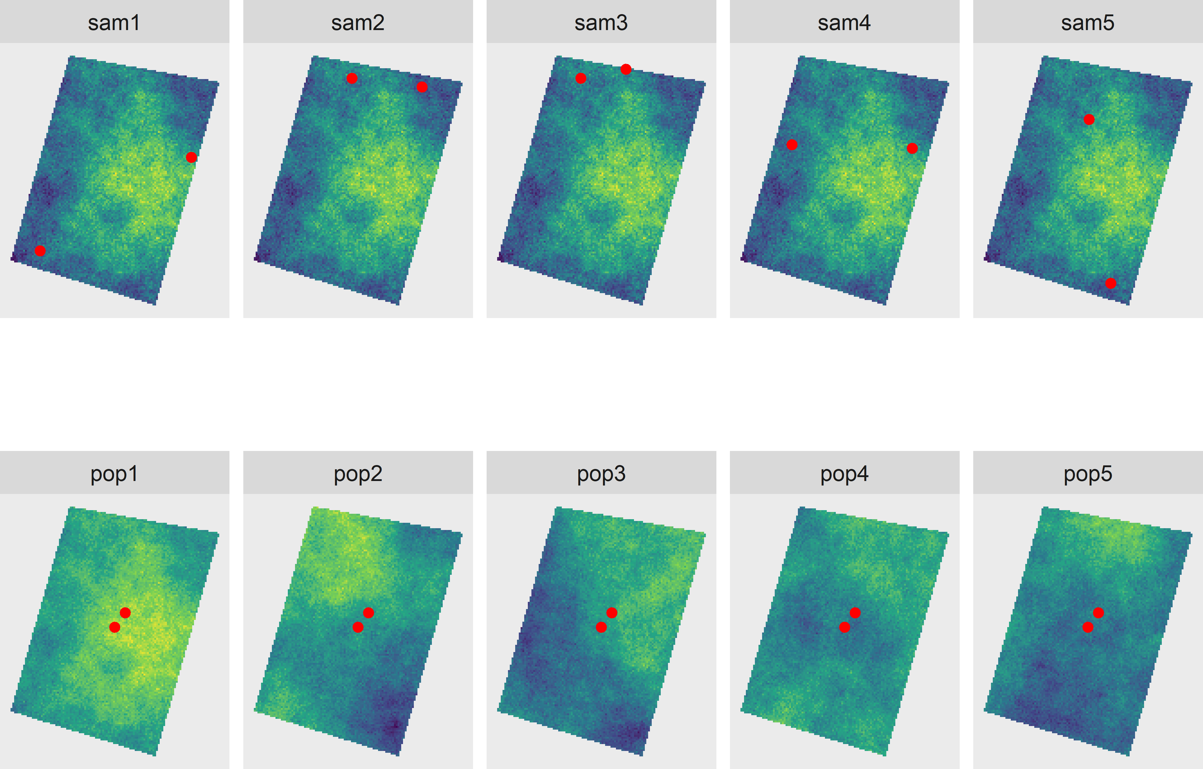
Figure 26.2: Illustration of independence in design-based and model-based approach. The top row shows five samples of two points selected randomly and independently from each other from one population (design-based approach). The bottom row shows two points not selected randomly, at a distance of 10 m from each other, from five model realisations (model-based approach).
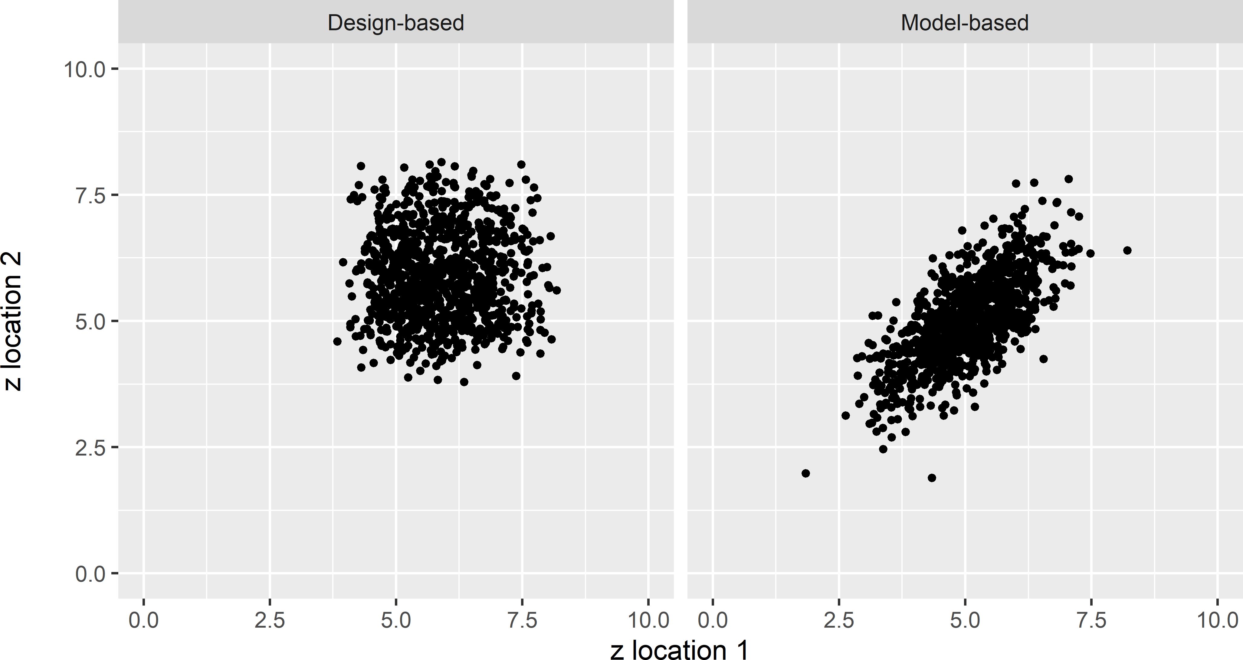
Figure 26.3: Scatter plots of the values of a study variable \(z\) at two randomly and independently selected points, 1,000 times selected from one population (design-based approach), and at two fixed points with a separation distance of 10 m, selected non-randomly from 1,000 model realisations (model-based approach).
The values measured at the two points are plotted against each other in a scatter plot, not for just five simple random samples or five populations, but for 1,000 samples and 1,000 populations (Figure 26.3). As we can see there is no correlation between the two variables generated by the repeated random selection of the two points (design-based), whereas the two variables generated by the repeated simulation of populations (model-based) are correlated.
Instead of two points, we may select two series of probability samples independently from each other, for instance two series of simple random samples (SI) of size 10, or two series of systematic random samples with random origin (SY) with an average size of 10, see Figure 26.4.
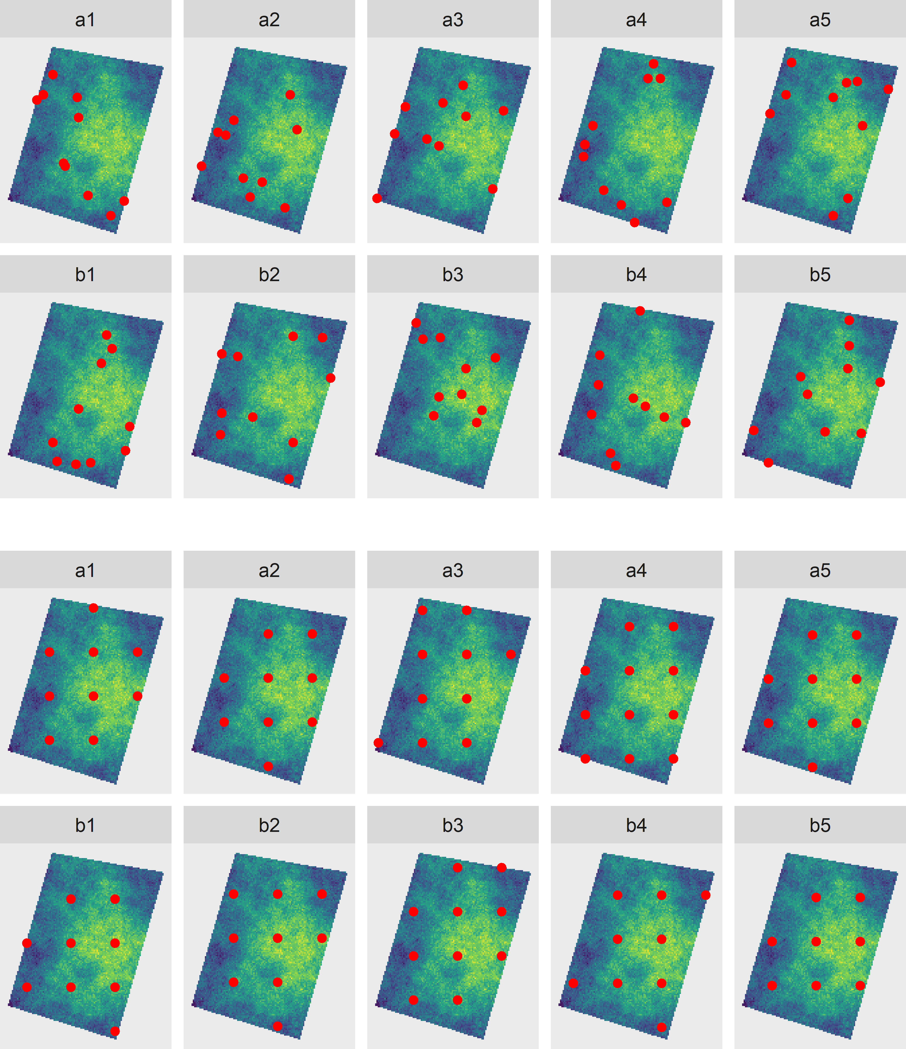
Figure 26.4: Two series (a and b) of simple random samples of ten points (top) and two series (a and b) of systematic random samples of, on average, ten points (bottom). The samples of series a and b are selected independently from each other.
Again, if we plot the sample means of pairs of simple random samples and pairs of systematic random samples against each other, we see that the two averages are not correlated (Figure 26.5). Note that the variation of the averages of the systematic random samples is considerably smaller than that of the simple random samples. The sampled population shows spatial structure. By spreading the sampling units over the spatial population, the precision of the estimated population mean is increased, see Chapter 5.
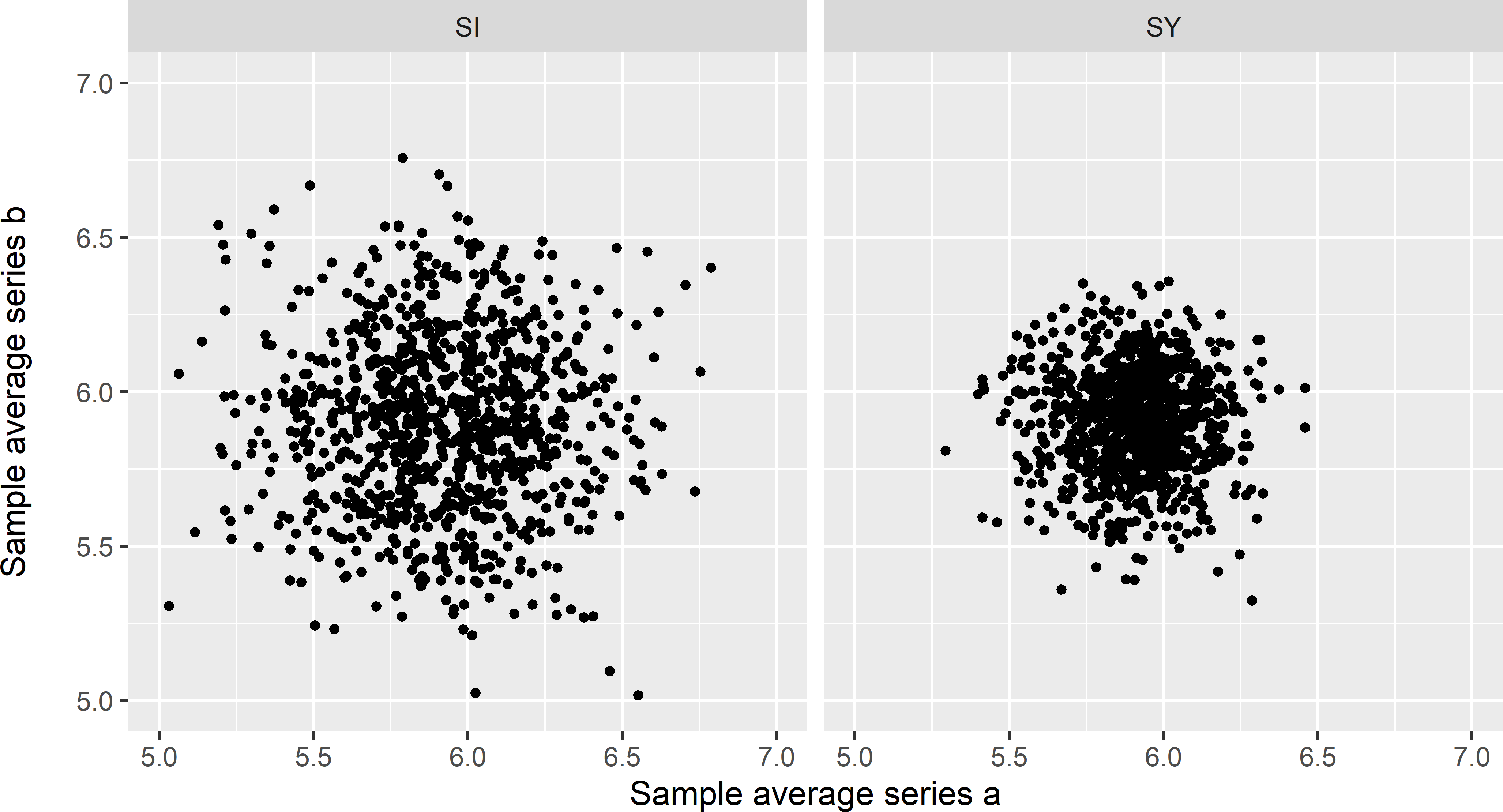
Figure 26.5: Scatter plots of averages of 1,000 pairs of simple random samples of ten points (SI) and of averages of 1,000 pairs of systematic random samples of ten points on average (SY).
This sampling experiment shows that independence is not a characteristic of a population, as stated by J. Wang et al. (2012), but of random variables generated by a random process (in the experiment the values at points or the sample means). As the random process differs between the design-based and the model-based approach, independence has a different meaning in these two approaches. For this reason, it is imperative to be more specific when using the term independence, by saying that data are design-independent or that you assume that the data are model-independent.
26.3 Bias and variance
Bias and variance are commonly used statistics to quantify the quality of an estimator. Bias quantifies the systematic error, variance the random error of the estimator. Both are defined as expectations. But are these expectations over realisations of a probability sampling design (samples) or realisations of a statistical model (populations)? Like independence, it is important to distinguish design-bias from model-bias and design-variance (commonly referred to as sampling variance) from model-variance.
The concept of model-unbiasedness deserves more attention. Figure 26.6 shows a preferential sample from a population simulated by sequential Gaussian simulation with a constant mean of 10 and an exponential semivariogram without nugget, a sill of 5, and a distance parameter of 20. The points are selected by sampling with draw-by-draw selection probabilities proportional to size (pps sampling, Chapter 8), using the square of the simulated values as a size variable. We may have a similar sample that is collected for delineating soil contamination or detecting hot spots of soil bacteria, etc. Many samples are selected at locations with a large value, few points at locations with a small value. The sample data are used in ordinary kriging (Figure 26.6). The prediction errors are computed by subtracting the kriged map from the simulated population.
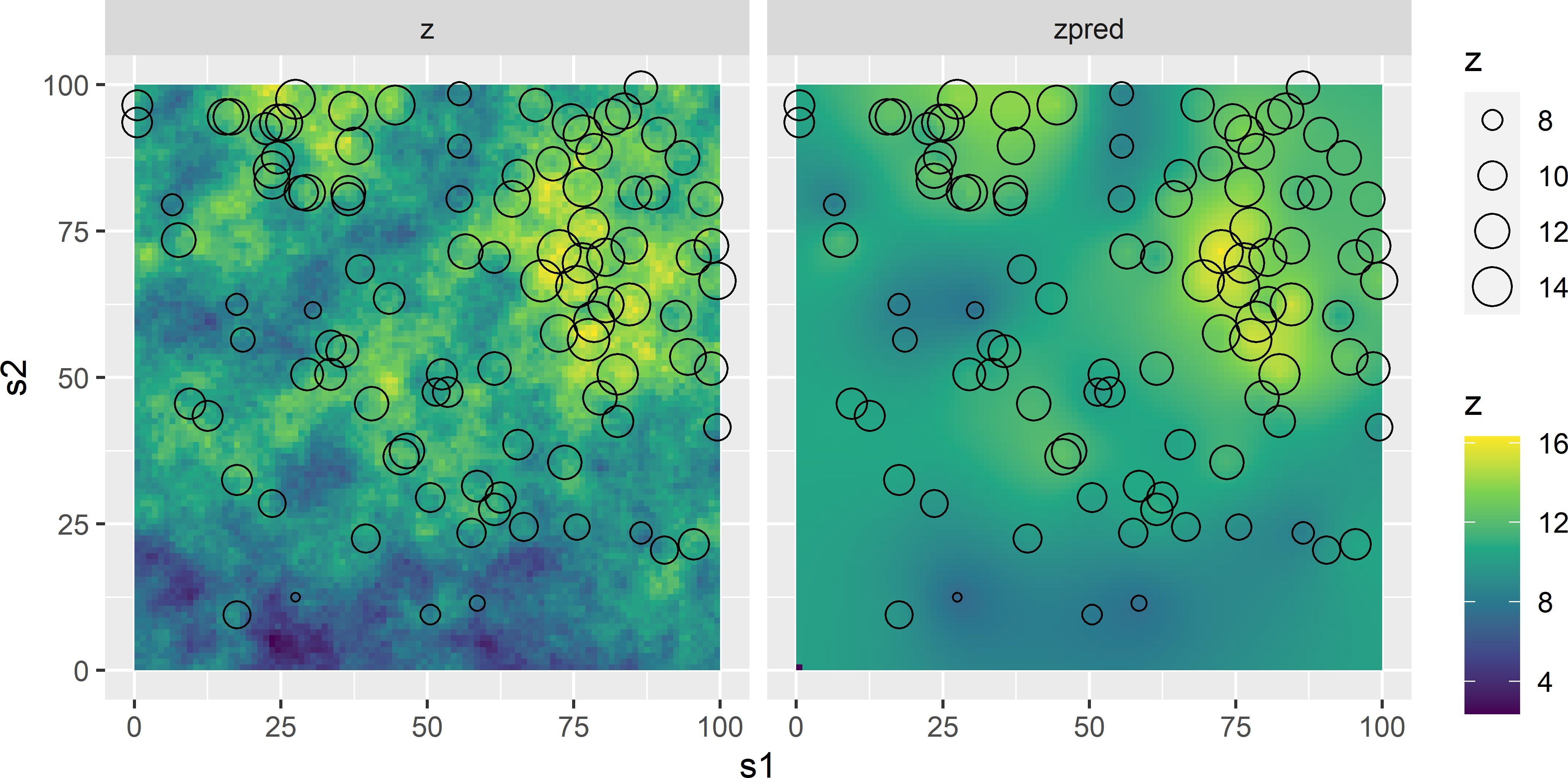
Figure 26.6: Preferential sample (size of open dots is proportional to value of study variable) from a simulated field (z) and map of ordinary kriging predictions (zpred).
Figure 26.7 shows a histogram of the prediction errors. The population mean error equals 0.482, not 0. You may have expected a positive systematic error because of the overrepresentation of locations with large values, but on the other hand, kriging predictions are best linear unbiased predictions (BLUP), so from that point of view, this systematic error might be unexpected. BLUP means that at individual locations the ordinary kriging predictions are unbiased. However, apparently this does not guarantee that the average of the prediction errors, averaged over all population units, equals 0. The reason is that unbiasedness is defined here over all realisations (populations) of the statistical model of spatial variation. So, the U in BLUP stands for model-unbiasedness. For other model realisations, sampled at the same points, we may have much smaller values, leading to a negative mean error of that population. On average, over all populations, the error at any point will be 0 and consequently also the average over all populations of the mean error.
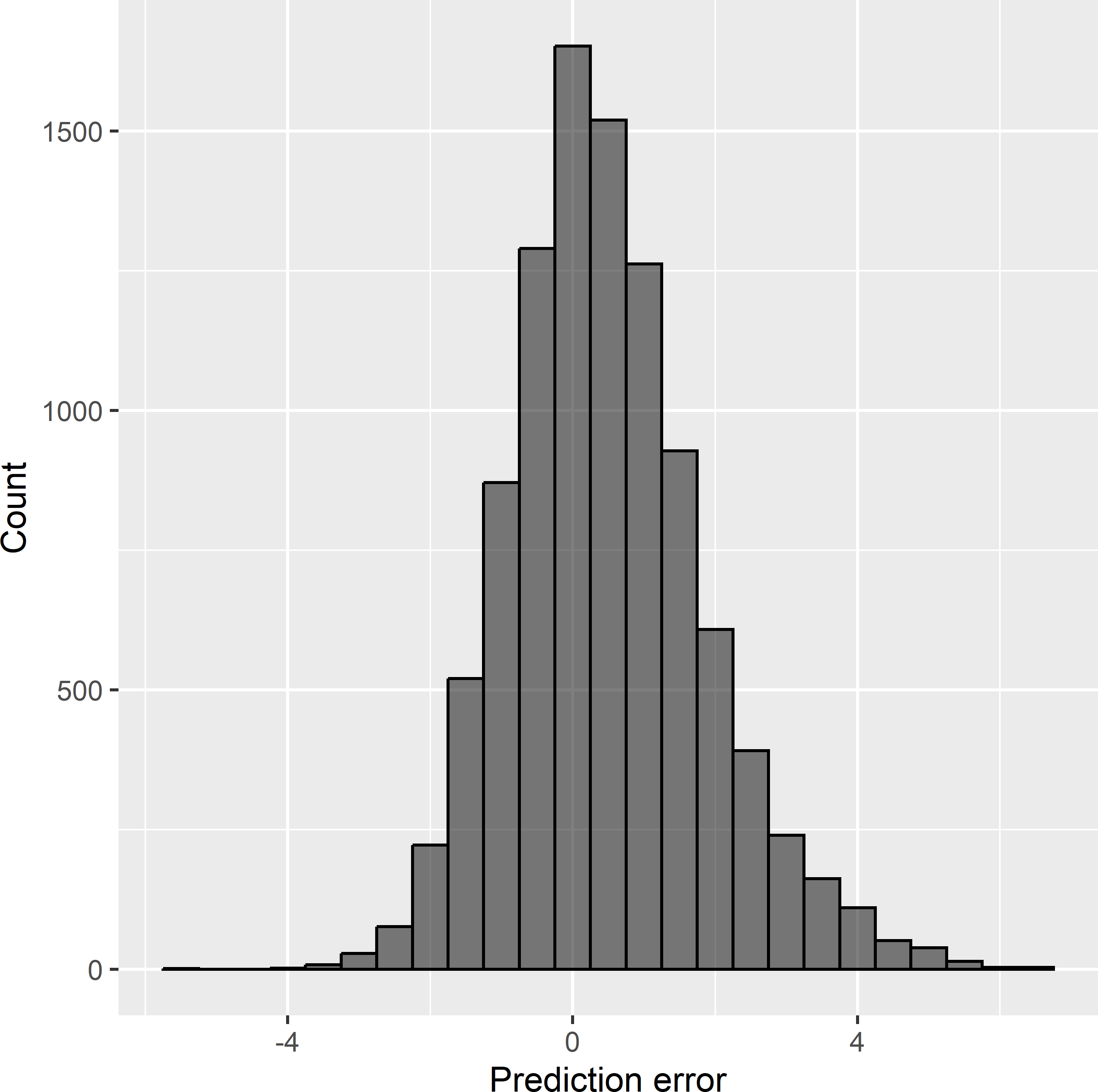
Figure 26.7: Frequency distribution of the errors of ordinary kriging predictions from a preferential sample.
This experiment shows that model-unbiasedness does not protect us against selection bias, i.e., bias due to preferential sampling.
26.4 Effective sample size
Another persistent misconception is that when estimating the variance of the estimator of the mean of a spatial population or the correlation of two variables of a population, we must account for autocorrelation of the sample data. This misconception occurs, for instance, in Griffith (2005) and in various sections (for instance, sections 3.5, 10.1, and 11.2) of Plant (2012). The reasoning is that, due to the spatial autocorrelation in the sample data, there is less information in the data about the parameter of interest, and so the effective sample size is smaller than the actual sample size. An early example of this misconception is Barnes’ publication on the required sample size for estimating nonparametric tolerance intervals (Barnes 1988). de Gruijter and ter Braak (1992) showed that a basic probability sampling design like simple random sampling requires fewer sampling points than the model-based sampling design proposed by Barnes.
The misconception is caused by confusing population parameters with model parameters. Recall that the population mean and the model-mean are not the same; the model-mean \(\mu\) of Equation (21.2) is the expectation of the population means over all populations that can be simulated with the model. The same holds for the variance of a variable as well as for the covariance and the Pearson correlation coefficient of two variables. All these parameters can be defined as parameters of a finite or infinite population or of random variables generated by a superpopulation model. Using an effective sample size to quantify the variance of an estimator is perfectly correct for model parameters, but not so for population parameters. For instance, when the correlation coefficient is defined as a population parameter and sampling units are selected by simple random sampling, there is no need to apply the method proposed by Clifford, Richardson, and Hémon (1989) to correct the p-value in a significance test for the presence of spatial autocorrelation.
I elaborate on this for the mean as the parameter of interest. Suppose a sample is selected in some way (need not be random) and the sample mean is used as an estimator of the model-mean. Note that for a model with a constant mean as in Equation (21.2), the sample mean is a model-unbiased estimator of the model-mean, but in general not the best linear unbiased estimator (BLUE) of the model-mean. If the random variables are model-independent, the variance of the sample mean, used as an estimator of the model-mean, can be computed by
\[\begin{equation} V(\hat{\mu}) = \frac{\sigma^2}{n} \;, \tag{26.2} \end{equation}\]
with \(\sigma^2\) the model-variance of the random variable (see Equation (21.2)). The variance presented in Equation (26.2) necessarily is a model-variance as it quantifies our uncertainty about the model-mean, which only exists in the model-based approach. If the random variables are not model-independent, the model-variance of the sample mean can be computed by (de Gruijter et al. 2006)
\[\begin{equation} V(\hat{\mu}) = \frac{\sigma^2}{n} \{1+(n-1)\bar{\rho}\} \;, \tag{26.3} \end{equation}\]
with \(\bar{\rho}\) the mean correlation within the sample (the average of the correlation of all pairs of sampling points). The term inside the curly brackets is larger than 1, unless \(\bar{\rho}\) equals 0. So, the variance of the estimator of the model-mean with dependent data is larger than when data are independent. The number of independent observations that is equivalent to a spatially autocorrelated data set’s sample size \(n\), referred to as the effective sample size, can be computed by (de Gruijter et al. 2006)
\[\begin{equation} n_{\mathrm{eff}}= \frac{n}{\{1+(n-1)\bar{\rho}\}} \;. \tag{26.4} \end{equation}\]
So, if we substitute \(n_{\mathrm{eff}}\) for \(n\) in Equation (26.2), we obtain the variance presented in Equation (26.3). Equation (26.4) is equivalent to equation (2) in Griffith (2005). Figure 26.8 shows that the effective sample size decreases sharply with the mean correlation. With a mean correlation of 0, the effective sample size equals the actual sample size; with a mean correlation of 1, the effective sample size equals 1.
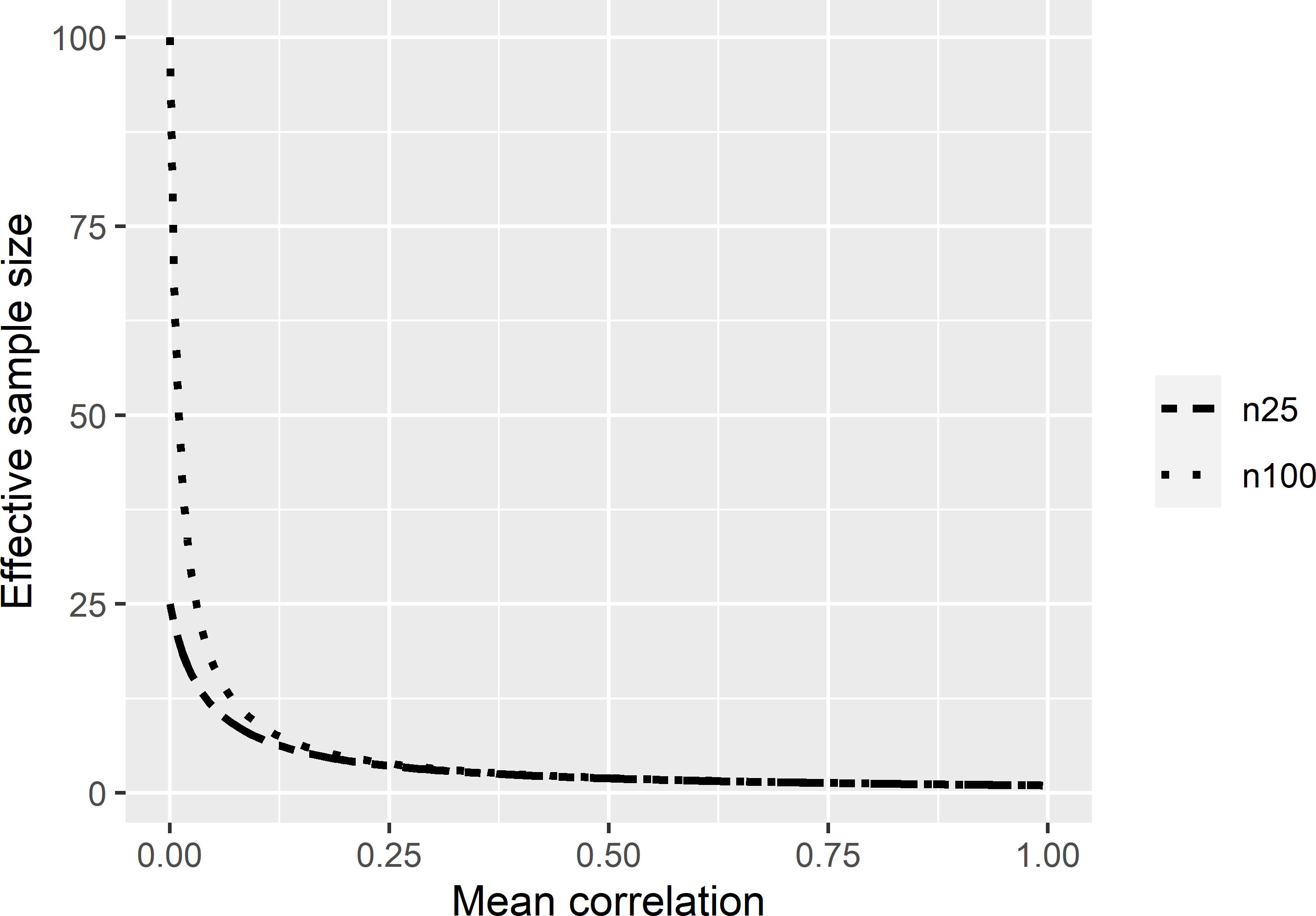
Figure 26.8: Effective sample sizes as a function of the mean correlation within the sample, for samples of size 25 and 100.
To illustrate the difference between the model-variance and the design-variance of a sample mean, I simulated a finite population of 100 units, located at the nodes of a square grid, with a model-mean of 10, an exponential semivariogram without nugget, an effective range of three times the distance between adjacent population units, and a sill of 1 (Figure 26.9). The model-variance of the average of a simple random sample without replacement of size \(n\) is computed using Equation (26.3), and the design-variance of the sample mean, used as an estimate of the population mean, is computed by (see Equation (3.11))
\[\begin{equation} V(\hat{\bar{z}})=\left(1-\frac{n}{N}\right)\frac{S^2}{n} \;, \tag{26.5} \end{equation}\]
with \(N\) the total number of population units (\(N=100\)). This is done for a range of sample sizes: \(n = 10, 11, \dots ,100\). Note that for \(n < 100\) the model-variance of the sample mean for a given \(n\), differs between samples. For samples showing strong spatial clustering, the mean correlation is relatively large, and consequently the model-variance is relatively large (see Equation (26.3)). There is less information in these samples about the model-mean than in samples without spatial clustering of the points. Therefore, to estimate the expectation of the model-variance over repeated simple random sampling for a given \(n\), I selected 200 simple random samples of that size \(n\), and I averaged the 200 model-variances. Figure 26.10 shows the result. Both the model-variance and the design-variance of the sample mean decrease with the sample size. For all sample sizes, the model-variance is larger than the design-variance. The design-variance goes to 0 for \(n = 100\) (see Equation (26.5)), whereas the model-variance for \(n = 100\) equals 0.0509. This can be explained as follows. Although with \(n = 100\) we know the population mean without error, this population mean is only an estimate of the model-mean. Recall that the model-mean is the expectation of the population mean over all realisations of the model.
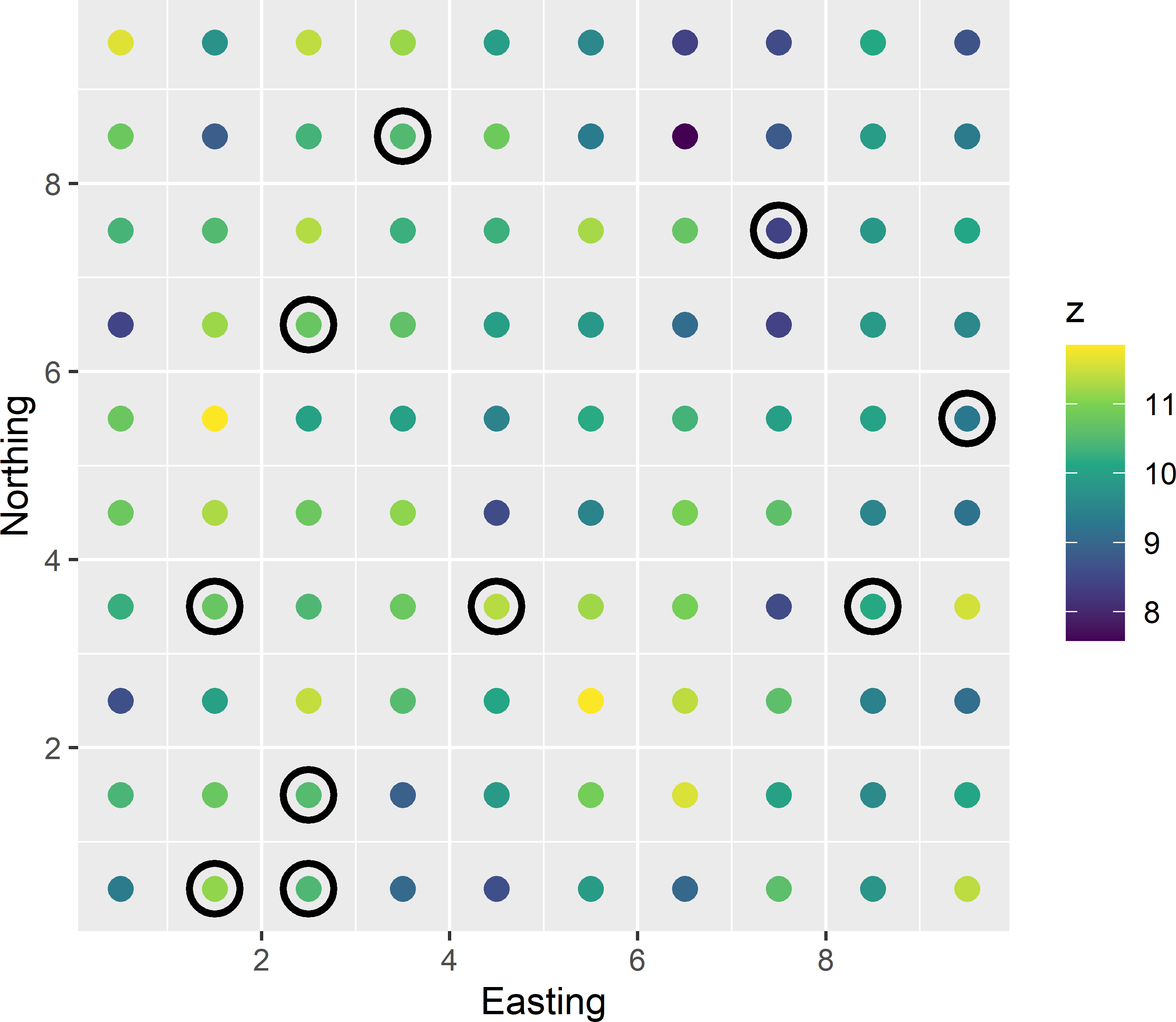
Figure 26.9: Simple random sample without replacement of ten points from a finite population simulated with a model with a model-mean of 10, a model-variance of 1, and an exponential semivariogram (without nugget) with a distance parameter equal to the distance between neighbours (effective range is three times this distance). The mean correlation within the sample equals 0.135, and the model-variance of the estimator of the model-mean equals 0.222.
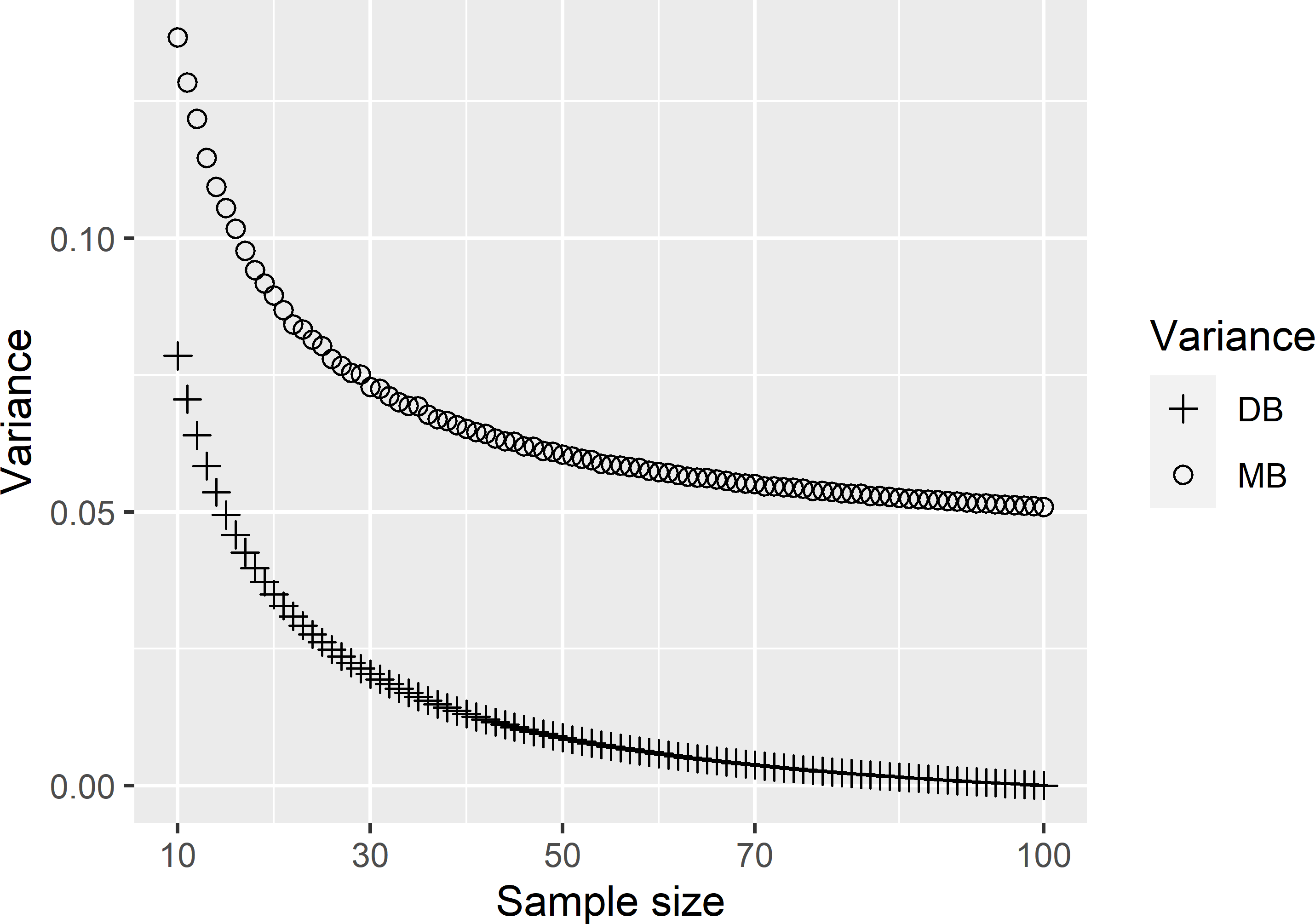
Figure 26.10: Model-variance (MB) and design-variance (DB) of the average of a simple random sample without replacement as a function of the sample size.
In Figure 26.11 we can see that the population mean shows considerable variation. The variance of 10,000 simulated population means equals 0.0513, which is nearly equal to the value of 0.0509 for the model-variance computed with Equation (26.3).
In observational research, I cannot think of situations in which interest is in estimation of the mean of a superpopulation model. This in contrast to experimental research. In experimental research, we are interested in the effects of treatments; think for instance of the effects of different types of soil tillage on the soil carbon stock. These treatment effects are quantified by different model-means. Also, in time-series analysis of data collected in observational studies, we might be more interested in the model-mean than in the mean over a bounded period of time.
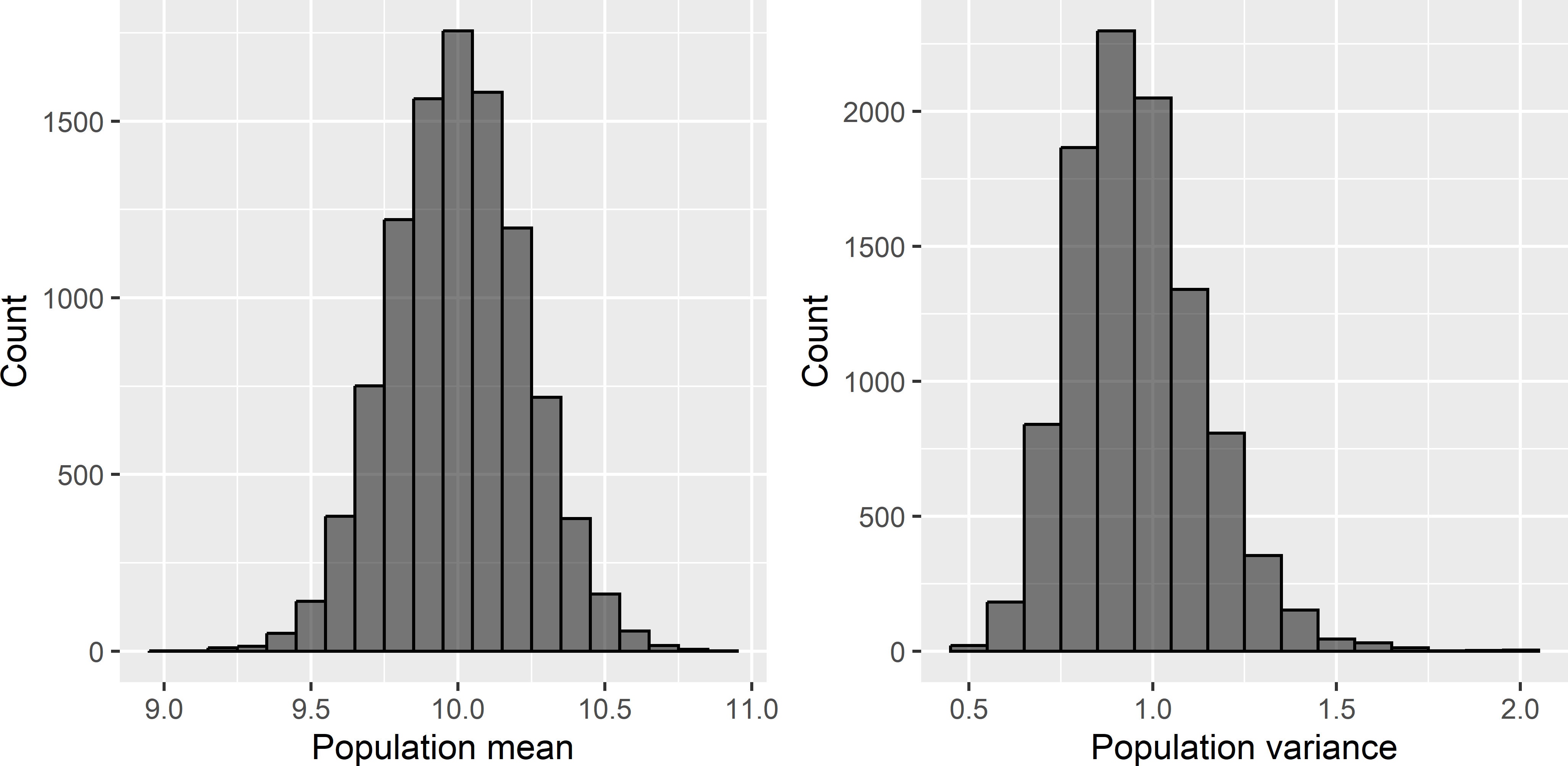
Figure 26.11: Frequency distributions of means and variances of 10,000 simulated populations.
Now let us return to Equation (26.1). What is wrong with this variance estimator? Where Griffith (2005) confused the population mean and the model-mean, J. Wang, Haining, and Cao (2010) confused the population variance with the sill (a priori variance) of the random process that has generated the population (Webster and Oliver 2007). The parameter \(\sigma^2\) in their formula is defined as the population variance. In doing so, the variance estimator is clearly wrong. However, if we define \(\sigma^2\) in this formula as the sill, the formula makes more sense, but even then, the equation is not fully correct. The variance computed with this equation is not the design-variance of the average of a simple random sample selected from the sampled population, but the expectation of this design-variance over all realisations of the model. So, it is a model-based prediction of the design-variance of the estimator of the population mean, estimated from a simple random sample, see Chapter 13. For the population actually sampled, the design-variance is either smaller or larger than this expectation. Figure 26.11 shows that there is considerable variation in the population variance among the 10,000 populations simulated with the model. Consequently, for an individual population, the variance of the estimator of the population mean, estimated from a simple random sample, can largely differ from the model-expectation of this variance. Do not use Equation (26.1) for estimating the design-variance of the estimator of the population mean, but simply use Equation (26.5) (for simple random sampling with replacement and simple random sampling of infinite populations the term \((1-n/N)\) can be dropped). Equation (26.1) is only relevant for comparing simple random sampling with other sampling designs under a variety of models of spatial variation, see Section 13.1.1 (Ripley (1981), Domburg, de Gruijter, and Brus (1994)).
26.5 Exploiting spatial structure in design-based approach
A further misconception is that, in the design-based approach, the possibilities of exploiting our knowledge about the spatial structure of the study variable are limited, because the sampling units are selected randomly. This would indeed be a very serious drawback, but happily enough, this is not true. There are various ways of utilising this knowledge. Our knowledge about the spatial structure can be used either at the stage of designing the sample and/or at the stage of the statistical inference once the data are collected (Table 26.1).
I distinguish the situation in which maps of covariates are available from the situation in which such maps are lacking. In the first situation, the covariate maps can be used, for instance, to stratify the population (Chapter 4). With a quantitative covariate, optimal stratification methods are available. Other options are, for instance, pps sampling (Chapter 8), and balanced sampling and well-spread sampling in covariate space with the local pivotal method (Chapter 9). At the inference stage, the covariate maps can be used in a model-assisted approach, using, for instance, a linear regression model to increase the precision of the design-based estimator (Chapter 10, Section 26.6).
If no covariate maps are available, we may anticipate the presence of spatial structure by spreading the sampling units throughout the study area. This spreading can be done in many ways, for instance by systematic random sampling (Chapter 5), compact geographical stratification (Section 4.6), well-spread sampling in geographical space with the local pivotal method (LPM) (Subsection 9.2.1), and generalised random-tessellation stratified (GRTS) sampling (Subsection 9.2.2). At the inference stage, again a model-assisted approach can be advantageous, using the spatial coordinates in a regression model.
| Stage | Covariates available | No covariates |
|---|---|---|
| Sampling | Stratified random sampling | Systematic random sampling |
| pps sampling | Compact geographical stratification | |
| Balanced sampling | Geographical spreading with LPM | |
| Covariate space spreading with LPM | GRTS sampling | |
| Inference | Model-assisted: regression model | Model-assisted: spatial regression model |
| LPM: local pivotal method. |
26.6 Model-assisted vs. model-dependent
In this section the difference between the model-assisted approach and the model-based approach is explained. The model-assisted approach is a hybrid approach in between the design-based and the model-based approach. It tries to build the strength of the model-based approach, a potential increase of the accuracy of estimates, into the design-based approach. As in the design-based approach, sampling units are selected by probability sampling, and consequently bias and variance are defined as design-bias and design-variance (Table 26.2). As in the model-based approach, a superpopulation model is used. However, the role of this model in the two approaches is fundamentally different. In both approaches we assume that the population of interest is a realisation of the superpopulation model. However, as explained above, in the model-based approach, the statistical properties of the estimators (predictors), such as bias and variance, are defined over all possible realisations of the model (Table 26.2). So, unbiasedness and minimum variance of an estimator (predictor) means model-unbiasedness and minimum model-variance. On the contrary, in the model-assisted approach, the model is used to derive an efficient estimator (Chapter 10). To stress its different role in the model-assisted approach, the model is referred to as a working model.
| Approach | Sampling | Inference | Regression coefficients | Quality criteria |
|---|---|---|---|---|
| Design-based | Prob. sampling | Design-based | No model | Design-bias, Design-variance |
| Model-assisted | Prob. sampling | Model-assisted | Population par. | Design-bias, Design-variance |
| Model-based | No requirement | Model-depend. | Superpop. par. | Model-bias, Model-variance |
An important property of model-assisted estimators is that, if a poor working model is used (our assumptions about how our population is generated are incorrect), then for moderate sample sizes the results are still valid, i.e., the empirical coverage rate of a model-assisted estimate of the confidence interval of the population mean still is approximately equal to the nominal coverage rate. This is because the mismatch of the superpopulation model and the applied model-assisted estimator results in a large design-variance of the estimator of the population mean. This is illustrated with a simulation study, in which I compare the effect of using a correct vs. an incorrect model in estimation.
A population is simulated with a simple linear regression model with an intercept of 15 (\(\beta_0 = 15\)), a slope coefficient of 0.5 (\(\beta_1 = 0.5\)), and a constant residual standard deviation of 2 (\(\sigma_{\epsilon}=2\)). This is done by first simulating a population with covariate values with a model-mean of 20 (\(\mu(x)=20\)), using an exponential semivariogram without nugget, a sill variance of 25, and a distance parameter of 20 distance units. This field with covariate values is then linearly transformed using the above-mentioned regression coefficients. Finally, `white noise’ is added by drawing independently for each population unit a random number from a normal distribution with zero mean and a standard deviation of 2 (Figure 26.12).
The population mean of the study variable equals 25.052, which is pretty close to the known model-mean \(\mu(z)\): \(\beta_0 + \beta_1 \mu(x)= 15 + 0.5 \cdot 20\).
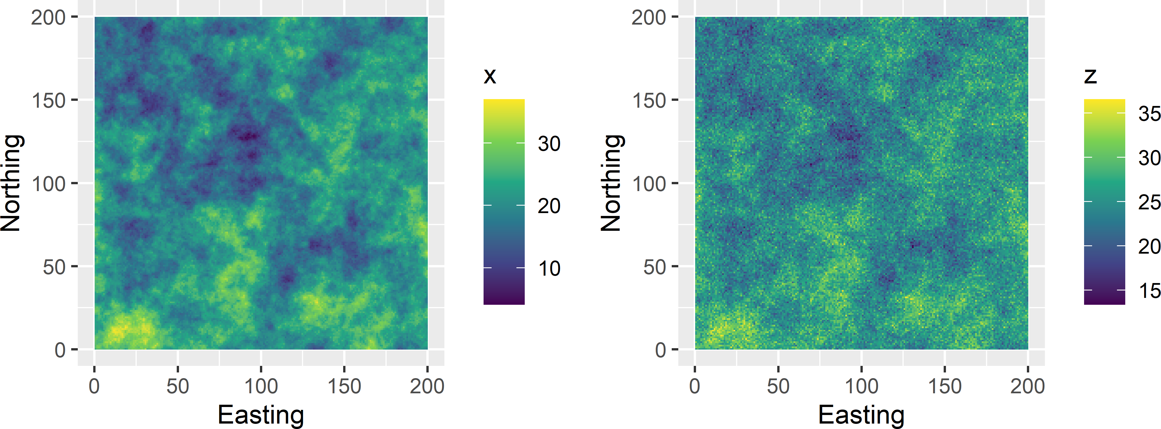
Figure 26.12: Realisation of simple linear regression model. x is the covariate, z is the study variable.
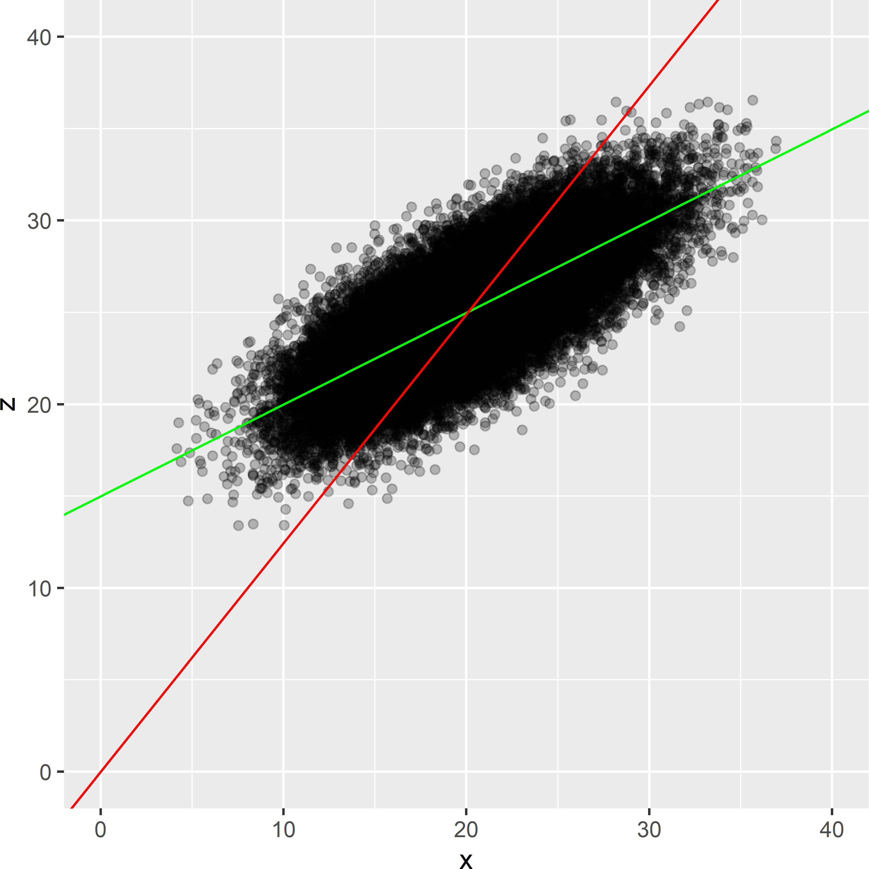
Figure 26.13: Exhaustive scatter plot of the simulated population, with population fit of a simple linear regression model (green line), and of a ratio model fitted with weights inversely proportional to the covariate (red line).
Figure 26.13 shows a scatter plot for all population units. The Pearson correlation coefficient equals 0.745. Two models are fitted to the exhaustive scatter plot: a simple linear regression model and a ratio model. The ratio model assumes that the intercept \(\beta_0\) equals 0 and that the residual variance is proportional to the covariate values: \(\sigma^2_{\epsilon} \propto x\). The population fits of the coefficients of the simple linear regression model are 14.9989 and 0.4997, which are very close to the model regression coefficients. The fitted ratio model is clearly very poor. The residual standard deviation of the population fit of the ratio model equals 3.887, which is much larger than 2.001 of the simple linear regression model.
The population mean of the study variable is estimated by selecting 5,000 times a simple random sample of 25 units. Each sample is used to estimate the population mean by two model-assisted estimators: the simple regression estimator and the ratio estimator (Chapter 10). The first estimator correctly assumes that the population is a realisation of a simple linear regression model, whereas the latter incorrectly assumes that it is a realisation of a ratio model. For each sample, the standard error of the two estimators are estimated as well, which is used to compute a 95% confidence interval of the population mean. Then the empirical coverage rate is computed, i.e., the proportion of samples for which the population mean is inside the 95% confidence interval. Ideally, this empirical coverage rate is equal to the nominal coverage rate of 0.95.
The coverage rates of the simple regression estimator and the ratio estimator equal 0.931 and 0.948, respectively. Both coverage rates are very close to the nominal coverage rate of 0.95. So, despite the fact that the ratio estimator assumes an improper superpopulation model, the estimated confidence interval is still valid. The price we pay for the invalid model assumption is not an overestimated coverage rate of a confidence interval, but an increased standard error of the estimated population mean. The average over the 5,000 samples of the estimated standard error of the regression estimator equals 0.387, whereas that of the ratio estimator equals 0.772. The larger standard error of the ratio estimator leads to wider confidence intervals, which explains that the coverage rate is still correct.
This sampling experiment is now repeated for samples sizes \(n=10, 25, 50 , 100\) and for confidence levels \(1-\alpha=0.01,0.02, \dots , 0.99\).
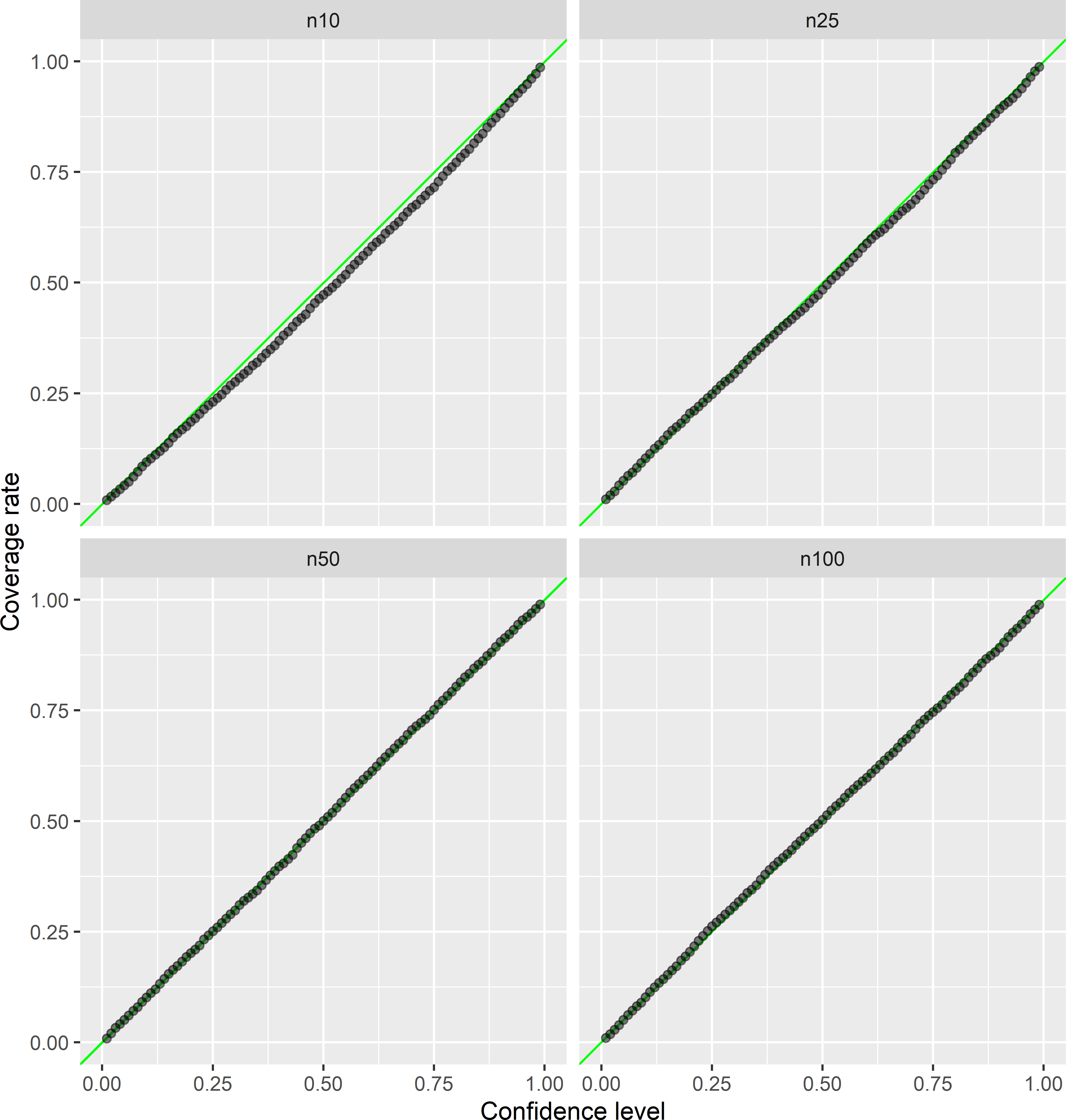
Figure 26.14: Empirical vs. nominal coverage rates of confidence intervals for the population mean, estimated by the simple regression estimator, for sample sizes 10, 25, 50, and 100.
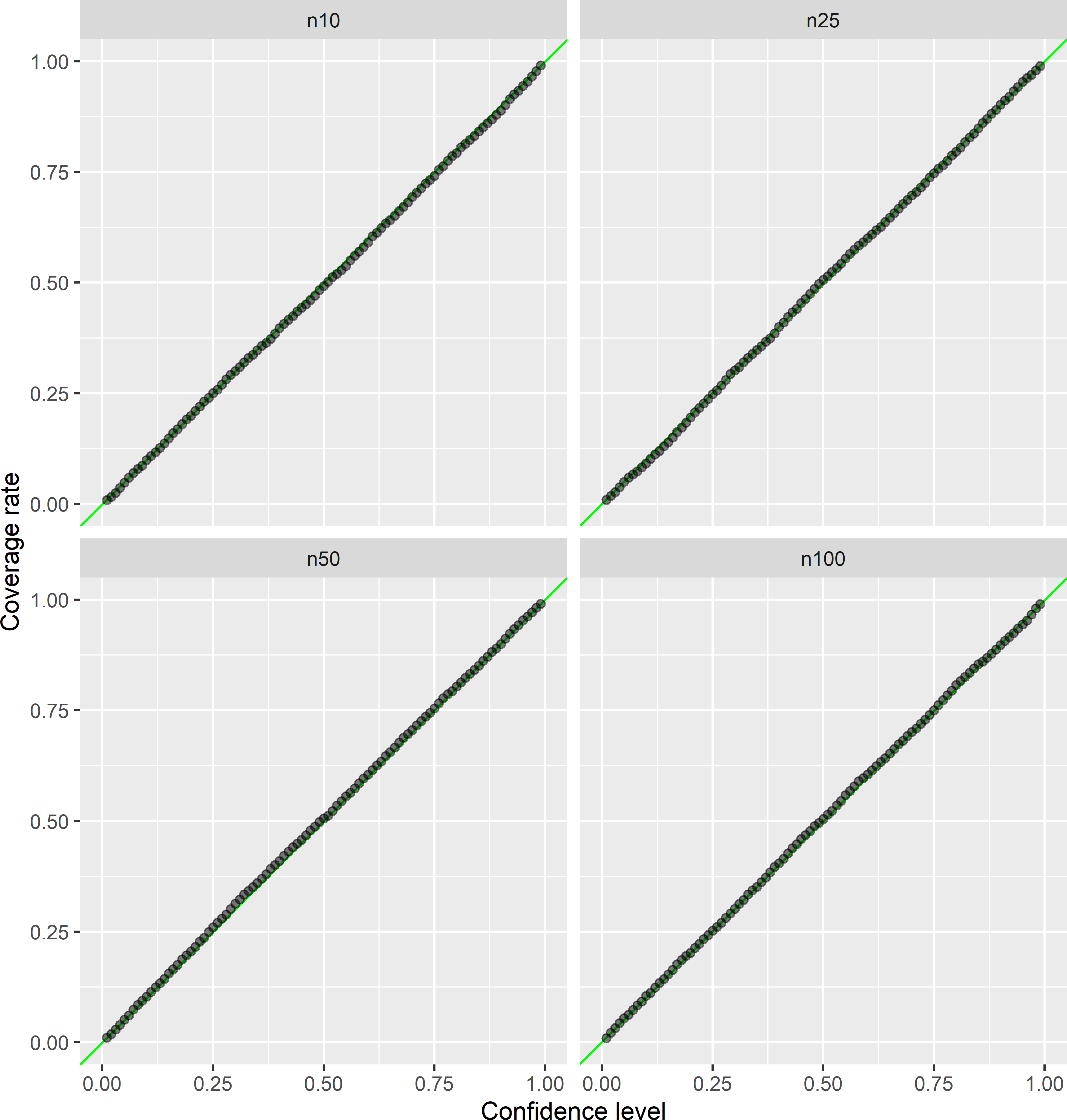
Figure 26.15: Empirical versus nominal coverage rates of confidence intervals for the population mean, estimated by the ratio estimator, for sample sizes 10, 25, 50, and 100.
| Estimator | n | Bias (%) | Standard deviation | Average standard error |
|---|---|---|---|---|
| Regression | 10 | 0.0037 | 0.678 | 0.609 |
| Regression | 25 | 0.0086 | 0.411 | 0.397 |
| Regression | 50 | 0.0172 | 0.282 | 0.282 |
| Regression | 100 | 0.0058 | 0.202 | 0.200 |
| Ratio | 10 | -0.3191 | 1.273 | 1.206 |
| Ratio | 25 | -0.1318 | 0.776 | 0.769 |
| Ratio | 50 | -0.0611 | 0.548 | 0.549 |
| Ratio | 100 | 0.0175 | 0.390 | 0.388 |
| n: sample size. |
Figures 26.14 and 26.15 show that the empirical coverage rates are close to the nominal coverage rate, for all four sample sizes, both estimators, and all confidence levels. For the regression estimator and \(n=10\), the empirical coverage rate is somewhat too small. This is because the standard error of the regression estimator is slightly underestimated at this sample size. The average of the estimated standard errors (square root of estimated variance of regression estimator) equals 0.609, which is somewhat smaller than the standard deviation of the 5,000 regression estimates of 0.678. For all sample sizes, the standard deviation of the 5,000 ratio estimates is considerably larger than that of the 5,000 regression estimates (Table 26.3). For \(n=10\) also the standard error of the ratio estimator is underestimated (the average of the 5,000 estimated standard errors is smaller than the standard deviation of the 5,000 ratio estimates), but as a percentage of the standard deviation of the 5,000 ratio estimates, this underestimation is smaller than for the regression estimator.
The relative bias, computed by
\[\begin{equation} bias = \frac{\frac{1}{5000}\sum_{s=1}^{5000} (\hat{\bar{z}}_s-\bar{z})}{\bar{z}} \;, \end{equation}\]
is about 0 for both estimators and all four sample sizes.
Contrarily, if in the model-based approach a poor superpopulation model is used, the predictions and the prediction error variances still are model-unbiased. However, for the sampled population, we may have serious systematic error in the estimated population mean and the variance of local predictions may be seriously over- or underestimated. For this reason, model-based inference is also referred to as model-dependent inference, stressing that we fully rely on the model and that the validity of the estimates and predictions depends on the quality of the model (Hansen, Madow, and Tepping 1983).