Chapter 14 Sampling for estimating parameters of domains
This chapter is about probability sampling and estimation of means or totals of subpopulations (subareas, subregions). In the sampling literature, these subpopulations are referred to as domains of interest, or shortly domains. Ideally, at the stage of designing a sample, these domains are known, and of every population unit we know to which domain it belongs. In that situation it is most convenient to use these domains as strata in random sampling, so that we can control the sample size in each domain (Chapter 4).
If we have multiple maps with domains, think for instance of a soil class map, a map with land cover classes, and a map with countries, we can make an overlay of these maps to construct the cross-tabulation strata. However, this may result in numerous strata, in some cases even more than the sample size. In this situation, an attractive solution is multiway stratification (Subsection 9.1.4). With this design, the domains of interest are used as strata, not their cross-classification, and the sample sizes of these marginal strata are controlled.
Even with a multiway stratified sample, resulting in controlled sample sizes for each domain, the sample size of a domain can be too small for a reliable estimate of the mean or total when using just the data of this domain. In this case we may use model-assisted estimators (Chapter 10) to increase the precision. Not only the data collected from a given domain are used to estimate the mean or total, but also data outside the domain (Section 14.2) (Chaudhuri (1994), Rao (2003), Falorsi and Righi (2008)).
We may also wish to estimate the mean or total of domains that are not used as strata or marginal strata. The sample size in these domains is then not controlled and varies among samples selected with the sampling design. As before with multiway stratified sampling, the mean can either be estimated with the direct estimator, using the data from the domain only (Section 14.1), or a model-assisted estimator, also using data from outside the domain (Section 14.2).
14.1 Direct estimator for large domains
If the sample size of a domain \(d\) is considered large enough to obtain a reliable estimate of the mean and, besides, the size of the domain is known, the mean of that domain can be estimated by the direct estimator:
\[\begin{equation} \hat{\bar{z}}_{d}=\frac{1}{N_{d}}\sum_{k \in \mathcal{S}_d}\frac{z_{dk}}{\pi _{dk}} \;, \tag{14.1} \end{equation}\]
where \(N_{d}\) is the size of the domain, \(z_{dk}\) is the value for unit \(k\) of domain \(d\), and \(\pi _{dk}\) is the inclusion probability of this point.
When the domain is not used as a (marginal) stratum, so that the sample size of the domain is random, the mean of the domain can be estimated best by the ratio estimator:
\[\begin{equation} \hat{\bar{z}}_{\text{ratio},d}= \frac{\hat{t}_d(z)}{\widehat{N}_d}= \frac{\sum_{k \in \mathcal{S}_d}\frac{z_{dk}}{\pi_{dk}}}{\sum_{k \in \mathcal{S}_d}\frac{1}{\pi_{dk}}} \;. \tag{14.2} \end{equation}\]
For simple random sampling without replacement, \(\pi_{dk} = n/N\). Inserting this in Equation (14.2) gives
\[\begin{equation} \hat{\bar{z}}_{\text{ratio},d}=\frac{1}{n_{d}}\sum_{k \in \mathcal{S}_d}z_{dk} \;. \tag{14.3} \end{equation}\]
The mean of the domain is simply estimated by the mean of the \(z\)-values observed in the domain, i.e., the sample mean in domain \(d\). The variance of this estimator can be estimated by
\[\begin{equation} \widehat{V}\!\left(\hat{\bar{z}}_{\text{ratio},d}\right) = \frac{1}{\hat{a}_{d}^{2}}\cdot\frac{1}{n\,(n-1)}\sum_{k \in \mathcal{S}_d}(z_{dk}-\bar{z}_{\mathcal{S}_d})^{2} \;, \tag{14.4} \end{equation}\]
where \(\bar{z}_{\mathcal{S}_d}\) is the sample mean in domain \(d\), and \(\hat{a}_{d}\) is the estimated relative size of domain \(d\):
\[\begin{equation} \hat{a}_{d}=\frac{n_{d}}{n} \;. \tag{14.5} \end{equation}\]
Refer to section (8.2.2) in de Gruijter et al. (2006) for the ratio estimator and its standard error with stratified simple random sampling, in case the domains cut across the strata, and other sampling designs.
The ratio estimator and its standard error can be computed with function svyby of package survey (Lumley 2021). This is illustrated with Eastern Amazonia. We wish to estimate the mean aboveground biomass (AGB) of the 16 ecoregions from a simple random sample of 200 units.
library(survey)
set.seed(314)
n <- 200
mysample <- grdAmazonia %>%
  mutate(N = n()) %>%
  slice_sample(n = n)
design_si <- svydesign(id = ~ 1, data = mysample, fpc = ~ N)
res <- svyby(~ AGB, by = ~ Ecoregion, design = design_si, FUN = svymean)
The ratio estimates of the mean AGB are shown in Table 14.1. Two ecoregions are missing in the table: no units are selected from these ecoregions so that a direct estimate is not available. There are three ecoregions with an estimated standard error of 0.0. These ecoregions have less than two sampling units only, so that the standard error cannot be estimated.
| Ecoregion | AGB | se |
|---|---|---|
| Cerrado | 99.7 | 15.6 |
| Guianan highland moist forests | 296.0 | 0.0 |
| Guianan lowland moist forests | 263.0 | 0.0 |
| Gurupa varzea | 80.0 | 0.0 |
| Madeira-Tapajos moist forests | 286.0 | 14.0 |
| Marajo varzea | 116.6 | 27.2 |
| Maranhao Babassu forests | 90.0 | 9.6 |
| Mato Grosso tropical dry forests | 177.0 | 90.7 |
| Monte Alegre varzea | 189.5 | 89.0 |
| Purus-Madeira moist forests | 145.5 | 47.1 |
| Tapajos-Xingu moist forests | 288.6 | 8.9 |
| Tocantins/Pindare moist forests | 176.3 | 17.9 |
| Uatuma-Trombetas moist forests | 274.7 | 6.7 |
| Xingu-Tocantins-Araguaia moist forests | 223.1 | 16.6 |
| The estimated standard errors of 0.0 are non-availables. |
The simple random sampling is repeated 1,000 times, and every sample is used to estimate the mean AGB of the ecoregions both with the \(\pi\) estimator and the ratio estimator. As can be seen in Table 14.2 the standard deviation of the ratio estimates is much smaller than that of the \(\pi\) estimates. The reason is that the number of sampling units in an ecoregion varies among samples, i.e., the sample size of an ecoregion is random. When many units are selected from an ecoregion, the estimated total of that ecoregion is large. The estimated mean as obtained with the \(\pi\) estimator then is large too, because the estimated total is divided by the fixed size (total number of population units, \(N_d\)) of the ecoregion. However, in the ratio estimator the size of an ecoregion is estimated from the same sample, although we know its size, see Equation (14.2). With many units selected from an ecoregion, the estimated size of that ecoregion, \(\widehat{N}_d\), is also large. By dividing the large estimated total by the large estimated size, a more stable estimate of the mean of the domain is obtained. For quite a few ecoregions the standard deviations are very large, especially of the \(\pi\) estimator. These are the ecoregions with very small average sample sizes. With simple random sampling, the expected sample size can simply be computed by \(E[n] = n \; N_d/N\). In the following section, alternative estimators are described for these ecoregions with small expected sample sizes. To speed up the computations, I used a 5 km \(\times\) 5 km subgrid of grdAmazonia in this sampling experiment.
| Ecoregion | HT | Ratio | n |
|---|---|---|---|
| Amazon-Orinoco-Southern Caribbean mangroves | 136.9 | 36.9 | 0.87 |
| Cerrado | 38.6 | 18.2 | 8.16 |
| Guianan highland moist forests | 271.4 | 29.5 | 0.71 |
| Guianan lowland moist forests | 160.0 | 17.9 | 2.51 |
| Guianan savanna | 101.5 | 67.1 | 2.86 |
| Gurupa varzea | 103.7 | 57.8 | 0.99 |
| Madeira-Tapajos moist forests | 55.9 | 14.2 | 22.96 |
| Marajo varzea | 48.6 | 24.7 | 10.80 |
| Maranhao Babassu forests | 59.3 | 25.7 | 4.61 |
| Mato Grosso tropical dry forests | 72.7 | 41.1 | 2.98 |
| Monte Alegre varzea | 120.2 | 63.3 | 2.27 |
| Purus-Madeira moist forests | 288.0 | 55.5 | 0.45 |
| Tapajos-Xingu moist forests | 45.5 | 12.0 | 31.51 |
| Tocantins/Pindare moist forests | 31.5 | 15.3 | 28.39 |
| Uatuma-Trombetas moist forests | 33.4 | 8.1 | 52.37 |
| Xingu-Tocantins-Araguaia moist forests | 42.4 | 17.2 | 27.56 |
| n: expected sample size. |
No covariates are used in the ratio estimator. If we wish to exploit covariates, the mean of a domain can be estimated best by the ratio of the regression estimate of the domain total and the estimated size of the domain:
\[\begin{equation} \hat{\bar{z}}_{\text{ratio},d}= \frac{\hat{t}_{\text{regr},d}(z)}{\widehat{N}_d}\;. \end{equation}\]
For a large domain with a reasonable sample size, the regression estimate can be computed from the data of that domain (Chapter 10). For small domains, also the data from outside these domains can be used to estimate the population regression coefficients. This is explained in Subsection 14.2.1.
14.2 Model-assisted estimators for small domains
When the domains are not well represented in the sample, the direct estimators from the previous section lead to large standard errors. In this situation, we may try to increase the precision by also using observations from outside the domain. If we have covariates related to the study variable, we may exploit this ancillary information by fitting a regression model relating the study variable to the covariates and using the fitted model to predict the study variable for all population units (nodes of discretisation grid), see Chapter 10. However, for a small domain, we may have too few sampled units in that domain to fit a separate regression model. The alternative then is to use the entire sample to estimate the regression coefficients, and to use this global regression model to estimate the means of the domains. This introduces a systematic error, a design-bias, in the estimator. However, this extra error is potentially outweighed by the reduction of the random error due to the use of the globally estimated regression coefficients. If one or more units are selected from a domain, the observations of the study variable of these units can be used to correct for the bias. This leads to the regression estimator for small domains. In the absence of such data, the mean of the domain can still be estimated by the so-called synthetic estimator.
There are quite a few packages for model-assisted estimation of means of small areas, the maSAE package (Cullman 2021), the JoSAE package (Johannes Breidenbach 2018), the rsae package (Schoch 2014), and the forestinventory package (Hill, Massey, and Mandallaz 2021). I use package forestinventory for model-assisted estimation (Subsections 14.2.1 and 14.2.2) and package JoSAE for model-based prediction of the means of small areas (Section 14.3).
14.2.1 Regression estimator
In the regression estimator, the potential bias due to the globally estimated regression coefficients can be eliminated by adding the \(\pi\) estimator of the mean of the regression residuals to the mean of the predictions in the domain (compare with Equation (10.8)) (Mandallaz (2007), Mandallaz, Breschan, and Hill (2013)):
\[\begin{equation} \hat{\bar{z}}_{\text{regr},d} = \frac{1}{N_d} \sum_{k=1}^{N_d} \mathbf{x}^{\mathrm{T}}_{dk} \hat{\mathbf{b}} + \frac{1}{N_d} \sum_{k \in \mathcal{S}_d} \frac{e_{dk}}{\pi_{dk}} = \bar{\mathbf{x}}_d^{\mathrm{T}} \hat{\mathbf{b}} + \frac{1}{N_d} \sum_{k \in \mathcal{S}_d} \frac{e_{dk}}{\pi_{dk}} \;, \tag{14.6} \end{equation}\]
with \(\mathbf{x}_{dk}\) the vector with covariate values for unit \(k\) in domain \(d\), \(\hat{\mathbf{b}}\) the vector with globally estimated regression coefficients, \(e_{dk}\) the residual for unit \(k\) in domain \(d\), \(\pi_{dk}\) the inclusion probability of that unit, and \(\bar{\mathbf{x}}_d\) the mean of the covariates in domain \(d\). Alternatively, the mean of the residuals in a domain is estimated by the ratio estimator:
\[\begin{equation} \hat{\bar{z}}_{\text{regr},d} = \bar{\mathbf{x}}_d^{\mathrm{T}} \hat{\mathbf{b}} + \frac{1}{\widehat{N}_d} \sum_{k \in \mathcal{S}_d} \frac{e_{dk}}{\pi_{dk}} \;, \tag{14.7} \end{equation}\]
with \(\widehat{N}_d\) the estimated size of domain \(d\), see Equation (14.2). The regression coefficients can be estimated by Equation (10.15). With simple random sampling, the second term in Equation (14.7) is equal to the sample mean of the residuals, so that the estimator reduces to
\[\begin{equation} \hat{\bar{z}}_{\text{regr},d}=\bar{\mathbf{x}}_d^{\mathrm{T}} \hat{\mathbf{b}} + \bar{e}_{\mathcal{S}_d}\;, \tag{14.8} \end{equation}\]
with \(\bar{e}_{\mathcal{S}_d}\) the sample mean of the residuals in domain \(d\).
A regression estimate can only be computed if we have at least one observation of the study variable in the domain \(d\). The variance of the regression estimator of the mean for a small domain can be estimated by (Hill, Massey, and Mandallaz 2021)
\[\begin{equation} \widehat{V}\!\left(\hat{\bar{z}}_{\text{regr},d}\right) = \bar{\mathbf{x}}_d^{\mathrm{T}} \widehat{\mathbf{C}}(\hat{\mathbf{b}}) \bar{\mathbf{x}}_d + \widehat{V}\!\left(\hat{\bar{e}}_d \right)\;, \tag{14.9} \end{equation}\]
with \(\widehat{\mathbf{C}}(\hat{\mathbf{b}})\) the matrix with estimated sampling variances and covariances of the estimators of the regression coefficients. The first variance component is the contribution due to uncertainty about the regression coefficients, the second component accounts for the uncertainty about the mean of the residuals in the domain. For simple random sampling, the sampling variance of the \(\pi\) estimator of the mean of the residuals in a domain can be estimated by the sample variance of the residuals in that domain divided by the sample size \(n_d\). This variance estimator is presented in Hill, Massey, and Mandallaz (2021). If the domain is not used as a stratum and the domain mean of the residuals is estimated by the ratio estimator, the second variance component can be estimated by
\[\begin{equation} \widehat{V}\!\left(\hat{\bar{e}}_{\text{ratio},d}\right) = \left(\frac{n}{n_{d}}\right)^{2}\cdot\frac{1}{n\,(n-1)}\sum_{k \in \mathcal{S}_d}(e_{dk}-\bar{e}_{\mathcal{S}_d})^{2} \;. \tag{14.10} \end{equation}\]
With simple random sampling, the sampling variances and covariances of the estimators of the regression coefficients can be estimated by (equation 2 in Hill, Massey, and Mandallaz (2021))
\[\begin{equation} \widehat{\mathbf{C}}(\hat{\mathbf{b}}) = \frac{1}{n} \left( \sum_{k \in \mathcal{S}} \mathbf{x}_k \mathbf{x}^{\mathrm{T}}_k \right) ^{-1} \left( \frac{1}{n^2} \sum_{k \in \mathcal{S}} e_k^2 \mathbf{x}_k \mathbf{x}^{\mathrm{T}}_k \right) \frac{1}{n}\left(\sum_{k \in \mathcal{S}}^n \mathbf{x}_k \mathbf{x}^{\mathrm{T}}_k \right)^{-1} \;. \tag{14.11} \end{equation}\]
The sampling variances and covariances of the estimators of the population regression coefficients are not equal to the model-variances and covariances as obtained with multiple linear regression, using functions lm and vcov, see Section 10.1 and Chapter 26.
Function twophase of package forestinventory (Hill, Massey, and Mandallaz 2021) can be used to compute the regression estimate for small domains and its standard error.
By assigning the domain means of the covariates to argument exhaustive of function twophase the sampling error of the first phase is ignored. Function twophase assumes simple random sampling (unless optional argument cluster is used). Note that for the unobserved population units (not selected units) the AGB values are changed into non-availables. In package survey also a function twophase is defined, for this reason the name of the package is made explicit by forestinventory::twophase. With argument psmall = TRUE and element unbiased = TRUE in the list small_area the regression estimate is computed. Log-transformed SWIR2 is used as a covariate in the regression estimator of the mean AGB of the ecoregions.
library(forestinventory)
n <- 200
set.seed(314)
units <- sample(nrow(grdAmazonia), size = n, replace = FALSE)
mysample <- grdAmazonia[units, c("AGB", "SWIR2", "Ecoregion")]
grdAmazonia <- grdAmazonia %>%
  mutate(lnSWIR2 = log(SWIR2),
         id = row_number(),
         ind = as.integer(id %in% units))
grdAmazonia$AGB[grdAmazonia$ind == 0L] <- NA
mx_eco_pop <- tapply(
  grdAmazonia$lnSWIR2, INDEX = grdAmazonia$Ecoregion, FUN = mean)
mX_eco_pop <- data.frame(
  Intercept = rep(1, length(mx_eco_pop)), lnSWIR2 = mx_eco_pop)
res <- forestinventory::twophase(AGB ~ lnSWIR2,
  data = as.data.frame(grdAmazonia),
  phase_id = list(phase.col = "ind", terrgrid.id = 1),
  small_area = list(sa.col = "Ecoregion",
                    areas = sort(unique(mysample$Ecoregion)),
                    unbiased = TRUE),
  psmall = TRUE, exhaustive = mX_eco_pop)
regr <- res$estimation| Ecoregion | AGB | ext_var | g_var | n2G |
|---|---|---|---|---|
| Cerrado | 105.5 | 51.6 | 82.6 | 12 |
| Guianan highland moist forests | 281.8 | NA | NaN | 1 |
| Guianan lowland moist forests | 280.3 | NA | NaN | 1 |
| Gurupa varzea | 57.8 | NA | NaN | 1 |
| Madeira-Tapajos moist forests | 296.1 | 91.2 | 107.3 | 19 |
| Marajo varzea | 163.1 | 535.2 | 546.0 | 10 |
| Maranhao Babassu forests | 114.2 | 157.1 | 178.1 | 7 |
| Mato Grosso tropical dry forests | 144.6 | 959.6 | 981.5 | 2 |
| Monte Alegre varzea | 209.1 | 4,105.7 | 4,117.3 | 2 |
| Purus-Madeira moist forests | 225.7 | 2,428.9 | 2,441.1 | 2 |
| Tapajos-Xingu moist forests | 277.8 | 23.4 | 36.9 | 38 |
| Tocantins/Pindare moist forests | 157.8 | 75.8 | 87.7 | 30 |
| Uatuma-Trombetas moist forests | 270.6 | 33.3 | 47.5 | 46 |
| Xingu-Tocantins-Araguaia moist forests | 223.6 | 51.1 | 61.6 | 29 |
| For explanation of variances of regression estimator, see text. n2G: sample size of ecoregion; NA: not available; NaN: not a number. |
The alternative is to save the selected units (sample) in a data frame, passed to function twophase with argument data. The results are identical because the true means of the covariate \(x\) specified with argument exhaustive contains all required information at the population level.
For two ecoregions, no regression estimate of the mean AGB is obtained (Table 14.3). No units are selected from these domains. The estimated variance of the estimated domain mean is in the column g_var. In the estimated variance ext_var the first variance component of Equation (14.9) is ignored. Note that for the ecoregions with a sample size of one unit (the sample size per domain is in column n2G), no estimate of the variance is available, because the variance of the estimated mean of the residuals cannot be estimated from one unit.
Figure 14.1 shows the regression estimates plotted against the ratio estimates. The intercept of the line, fitted with ordinary least squares (OLS), is larger than 0, and the slope is smaller than 1. Using the regression model predictions in the estimation of the means leads to some smoothing.
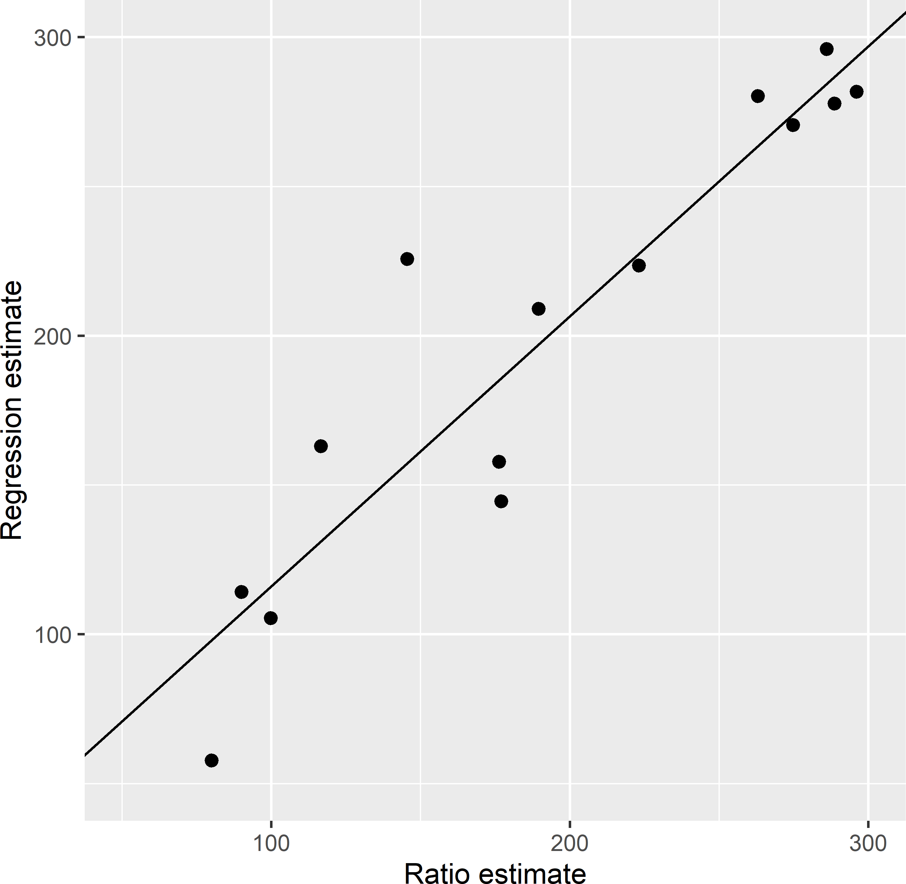
Figure 14.1: Scatter plot of the ratio and the regression estimates of the mean AGB (109 kg ha-1) of ecoregions in Eastern Amazonia for simple random sample without replacement of size 200. In the regression estimate, lnSWIR2 is used as a predictor. The line is fitted by ordinary least squares.
I quantified the gain in precision of the estimated mean AGB due to the use of the regression model by the variance of the ratio estimator divided by the variance of the regression estimator (Table 14.4). For ratios larger than 1, there is a gain in precision. Both variances are estimated from 1,000 repeated ratio and regression estimates obtained with simple random sampling without replacement of size 200. For all but two small ecoregions, there is a gain. For quite a few ecoregions, the gain is quite large. These are the ecoregions where the globally fitted regression model explains a large part of the spatial variation of AGB.
| Ecoregion | Gain |
|---|---|
| Amazon-Orinoco-Southern Caribbean mangroves | 0.57 |
| Cerrado | 1.63 |
| Guianan highland moist forests | 1.01 |
| Guianan lowland moist forests | 1.26 |
| Guianan savanna | 6.70 |
| Gurupa varzea | 0.65 |
| Madeira-Tapajos moist forests | 1.44 |
| Marajo varzea | 1.87 |
| Maranhao Babassu forests | 1.70 |
| Mato Grosso tropical dry forests | 2.81 |
| Monte Alegre varzea | 1.21 |
| Purus-Madeira moist forests | 1.74 |
| Tapajos-Xingu moist forests | 2.73 |
| Tocantins/Pindare moist forests | 2.56 |
| Uatuma-Trombetas moist forests | 2.10 |
| Xingu-Tocantins-Araguaia moist forests | 4.06 |
14.2.2 Synthetic estimator
For small domains from which no units are selected, the mean can still be estimated by the synthetic estimator, also referred to as the synthetic regression estimator, by dropping the second term in Equation (14.6):
\[\begin{equation} \hat{\bar{z}}_{\text{syn},d}=\bar{\mathbf{x}}_d^{\mathrm{T}} \hat{\mathbf{b}}\;. \tag{14.12} \end{equation}\]
The variance can be estimated by
\[\begin{equation} \widehat{V}\!\left(\hat{\bar{z}}_{\text{syn},d}\right) = \bar{\mathbf{x}}_d^{\mathrm{T}} \widehat{\mathbf{C}}(\hat{\mathbf{b}}) \bar{\mathbf{x}}_d \;. \tag{14.13} \end{equation}\]
This is equal to the first variance component of Equation (14.9).
The synthetic estimate can be computed with function twophase, with argument psmall = FALSE and element unbiased = FALSE in the list small_area.
res <- forestinventory::twophase(AGB ~ lnSWIR2,
  data = as.data.frame(grdAmazonia),
  phase_id = list(phase.col = "ind", terrgrid.id = 1),
  small_area = list(sa.col = "Ecoregion", areas = ecoregions, unbiased = FALSE),
  psmall = FALSE, exhaustive = mX_eco_pop)
synt <- res$estimation| Ecoregion | AGB | g_var | n2G |
|---|---|---|---|
| Amazon-Orinoco-Southern Caribbean mangroves | 225.3 | 10.6 | 0 |
| Cerrado | 81.6 | 31.0 | 12 |
| Guianan highland moist forests | 278.6 | 16.0 | 1 |
| Guianan lowland moist forests | 277.3 | 15.8 | 1 |
| Guianan savanna | 171.8 | 12.2 | 0 |
| Gurupa varzea | 218.2 | 10.4 | 1 |
| Madeira-Tapajos moist forests | 279.2 | 16.1 | 19 |
| Marajo varzea | 230.6 | 10.8 | 10 |
| Maranhao Babassu forests | 118.3 | 20.9 | 7 |
| Mato Grosso tropical dry forests | 114.0 | 21.9 | 2 |
| Monte Alegre varzea | 242.6 | 11.6 | 2 |
| Purus-Madeira moist forests | 250.4 | 12.3 | 2 |
| Tapajos-Xingu moist forests | 261.1 | 13.4 | 38 |
| Tocantins/Pindare moist forests | 175.7 | 11.9 | 30 |
| Uatuma-Trombetas moist forests | 267.2 | 14.2 | 46 |
| Xingu-Tocantins-Araguaia moist forests | 221.9 | 10.5 | 29 |
| n2G: sample size of ecoregion. |
For all ecoregions, also the unsampled ones, a synthetic estimate of the mean AGB is obtained (Table 14.5). For the sampled ecoregions, the synthetic estimate differs from the regression estimate. This difference can be quite large for ecoregions with a small sample size. Averaged over all sampled ecoregions, the difference, computed as synthetic estimate minus regression estimate, equals 14.9 109 kg ha-1. The variance of the regression estimator is always much larger than the variance of the synthetic estimator. The difference is the variance of the estimator of the domain mean of the residuals. However, recall that the regression estimator is design-unbiased, whereas the synthetic estimator is not. A more fair comparison is on the basis of the root mean squared error (RMSE) (Table 14.6). For the regression estimator, the RMSE is equal to its standard error and therefore not shown in the table.
| Ecoregion | RMSE reg | se syn | bias syn | RMSE syn |
|---|---|---|---|---|
| Amazon-Orinoco Carib. mangroves | 48.8 | 3.7 | 96.2 | 96.3 |
| Cerrado | 14.2 | 7.1 | -17.3 | 18.7 |
| Guianan highland moist forests | 29.4 | 4.9 | -1.2 | 5.0 |
| Guianan lowland moist forests | 15.9 | 4.8 | -7.2 | 8.7 |
| Guianan savanna | 25.9 | 4.1 | 12.3 | 13.0 |
| Gurupa varzea | 71.8 | 3.7 | 119.4 | 119.5 |
| Madeira-Tapajos moist forests | 11.8 | 4.9 | -2.2 | 5.4 |
| Marajo varzea | 18.1 | 3.8 | 74.4 | 74.5 |
| Maranhao Babassu forests | 19.7 | 5.7 | 3.9 | 6.9 |
| Mato Grosso tropical dry forests | 24.5 | 5.8 | 3.4 | 6.7 |
| Monte Alegre varzea | 57.5 | 3.9 | 50.6 | 50.8 |
| Purus-Madeira moist forests | 42.1 | 4.2 | 32.9 | 33.1 |
| Tapajos-Xingu moist forests | 7.3 | 4.4 | -18.5 | 19.0 |
| Tocantins/Pindare moist forests | 9.5 | 4.0 | 14.7 | 15.3 |
| Uatuma-Trombetas moist forests | 5.6 | 4.5 | -14.2 | 14.9 |
| Xingu-Toc.-Arag. moist forests | 8.5 | 3.7 | -2.5 | 4.4 |
In the synthetic estimator and the regression estimator, both quantitative covariates and categorical variables can be used. If one or more categorical variables are included in the estimator, the variable names in the data frame with the true means of the ancillary variables per domain, specified with argument exhaustive, must correspond to the column names of the design matrix that is generated with function lm, see Subsection 10.1.3.
14.3 Model-based prediction
The alternative for design-based and model-assisted estimation of the means or totals of small domains is model-based prediction. The fundamental difference between model-assisted estimation and model-based prediction is explained in Chapter 26. The models used in this section are linear mixed models. In a linear mixed model, the mean of the study variable is modelled as a linear combination of covariates, similar to a linear regression model. The difference with a linear regression model is that the residuals of the mean are not assumed independent. The dependency of the residuals is also modelled. Two types of linear mixed model are described: a random intercept model and a geostatistical model.
14.3.1 Random intercept model
A basic linear mixed model that can be used for model-based prediction of means of small domains is the random intercept model:
\[\begin{equation} \begin{split} Z_{dk} &= \mathbf{x}_{dk}^{\text{T}} \pmb{\beta} + v_d + \epsilon_{dk} \\ v_d &\sim \mathcal{N}(0,\sigma^2_v) \\ \epsilon_{dk} &\sim \mathcal{N}(0,\sigma^2_{\epsilon}) \;. \end{split} \tag{14.14} \end{equation}\]
Two random variables are now involved, both with a normal distribution with mean zero: \(v_d\), a random intercept at the domain level with variance \(\sigma^2_v\), and the residuals \(\epsilon_{dk}\) at the unit level with variance \(\sigma^2_{\epsilon}\). The variance \(\sigma^2_v\) can be interpreted as a measure of the heterogeneity among the domains after accounting for the fixed effect (J. Breidenbach and Astrup 2012). With this model, the mean of a domain can be predicted by
\[\begin{equation} \hat{\bar{z}}_{\text{mb},d} = \bar{\mathbf{x}}_d^{\mathrm{T}} \hat{\pmb{\beta}} + \hat{v}_d \;, \tag{14.15} \end{equation}\]
with \(\hat{\pmb{\beta}}\) the best linear unbiased estimates (BLUE) of the regression coefficients and \(\hat{v}_d\) the best linear unbiased prediction (BLUP) of the intercept for domain \(d\), \(v_d\). The model-based predictor can also be written as
\[\begin{equation} \hat{\bar{z}}_{\text{mb},d} = \bar{\mathbf{x}}_d^{\mathrm{T}} \hat{\pmb{\beta}} + \lambda_d \left( \frac{1}{n_d }\sum_{k \in \mathcal{S}_d} \epsilon_{dk} \right) \;, \tag{14.16} \end{equation}\]
with \(\lambda_d\) a weight for the second term that corrects for the bias of the synthetic estimator. This weight is computed by
\[\begin{equation} \lambda_d = \frac{\hat{\sigma}^2_v}{\hat{\sigma}^2_v + \hat{\sigma}^2_{\epsilon}/n_d}\;. \tag{14.17} \end{equation}\]
This equation shows that the larger the estimated residual variance \(\hat{\sigma}^2_{\epsilon}\), the smaller the weight for the bias correction factor, and the larger the sample size \(n_d\), the larger the weight. Comparing Equations (14.15) and (14.16) shows that the random intercept of a domain is predicted by the sample mean of the residuals of that domain, multiplied by a weight factor computed by Equation (14.17).
The means of the small domains can be computed with function eblup.mse.f.wrap of package JoSAE (Johannes Breidenbach 2018). It requires as input a linear mixed model generated with function lme of package nlme (Pinheiro et al. 2021). The simple random sample of size 200 selected before is used to fit the linear mixed model, with lnSWIR2 as a fixed effect, i.e., the effect of lnSWIR2 on the mean AGB. The random effect is added by assigning another formula to argument random. The formula ~ 1 | Ecoregion means that the intercept is treated as a random variable and that it varies among the ecoregions. This linear mixed model is referred to as a random intercept model: the intercepts are allowed to differ among the small domains, whereas the effects of the covariates, lnSWIR2 in our case, is equal for all domains.
Tibble grdAmazonia is converted to a data.frame to avoid problems with function eblup.mse.f.wrap hereafter. A simple random sample with replacement of size 200 is selected.
grdAmazonia <- grdAmazonia %>%
  as.data.frame() %>%
  mutate(x1 = x1 /1000,
         x2 = x2 / 1000)
set.seed(314)
mysample <- grdAmazonia %>%
  dplyr::select(x1, x2, AGB, lnSWIR2, Ecoregion) %>%
slice_sample(n = n, replace = TRUE)library(nlme)
library(JoSAE)
lmm_AGB <- lme(fixed = AGB ~ lnSWIR2, data = mysample, random = ~ 1 | Ecoregion)The fixed effects of the linear mixed model can be extracted with function fixed.effects.
The fixed effects of the linear mixed model differ somewhat from the fixed effects in the simple linear regression model (fixed_lm):
             fixed_lm fixed_lmm
(Intercept) 1778.1959 1667.9759
lnSWIR2     -241.1567 -225.6561
The random effect can be extracted with function random.effects.
                                       (Intercept)
Cerrado                                  21.439891
Guianan highland moist forests            6.397816
Guianan lowland moist forests             5.547995
Gurupa varzea                           -52.985839
Madeira-Tapajos moist forests            27.479921
Marajo varzea                           -50.587786
Maranhao Babassu forests                 -1.702322
Mato Grosso tropical dry forests         18.812207
Monte Alegre varzea                     -12.201148
Purus-Madeira moist forests              -9.320683
Tapajos-Xingu moist forests              28.760508
Tocantins/Pindare moist forests          -8.940962
Uatuma-Trombetas moist forests           16.165017
Xingu-Tocantins-Araguaia moist forests   11.135385
The random intercepts are added to the fixed intercept; the coefficient of lnSWIR2 is the same for all ecoregions:
                                       (Intercept)   lnSWIR2
Cerrado                                   1689.416 -225.6561
Guianan highland moist forests            1674.374 -225.6561
Guianan lowland moist forests             1673.524 -225.6561
Gurupa varzea                             1614.990 -225.6561
Madeira-Tapajos moist forests             1695.456 -225.6561
Marajo varzea                             1617.388 -225.6561
Maranhao Babassu forests                  1666.274 -225.6561
Mato Grosso tropical dry forests          1686.788 -225.6561
Monte Alegre varzea                       1655.775 -225.6561
Purus-Madeira moist forests               1658.655 -225.6561
Tapajos-Xingu moist forests               1696.736 -225.6561
Tocantins/Pindare moist forests           1659.035 -225.6561
Uatuma-Trombetas moist forests            1684.141 -225.6561
Xingu-Tocantins-Araguaia moist forests    1679.111 -225.6561
The fitted model can now be used to predict the means of the ecoregions as follows. As a first step, a data frame must be defined, with the size and the population mean of the covariate lnSWIR2 per domain. This data frame is passed to function eblup.mse.f.wrap with argument domain.data. This function computes the model-based prediction, as well as the regression estimator (Equation (14.6)) and the synthetic estimator (Equation (14.12)) and their variances. The model-based predictor is the variable EBLUP in the output data frame. For the model-based predictor, two standard errors are computed, see J. Breidenbach and Astrup (2012) for details.
N_eco <- tapply(grdAmazonia$AGB, INDEX = grdAmazonia$Ecoregion, FUN = length)
df_eco <- data.frame(Ecoregion = ecoregions, N = N_eco, lnSWIR2 = mx_eco_pop)
res <- eblup.mse.f.wrap(domain.data = df_eco, lme.obj = lmm_AGB)
df <- data.frame(Ecoregion = res$domain.ID, mb = res$EBLUP,
  se.1 = res$EBLUP.se.1, se.2 = res$EBLUP.se.2)
Table 14.7 shows the model-based predictions and the estimated standard errors of the mean AGB of the ecoregions, obtained with the random intercept model.
| Ecoregion | AGB | se.1 | se.2 |
|---|---|---|---|
| Cerrado | 101.9 | 11.4 | 11.5 |
| Guianan highland moist forests | 271.1 | 25.8 | 26.4 |
| Guianan lowland moist forests | 269.1 | 25.8 | 26.4 |
| Gurupa varzea | 155.3 | 36.0 | 31.8 |
| Madeira-Tapajos moist forests | 292.8 | 9.3 | 9.3 |
| Marajo varzea | 169.3 | 13.6 | 13.2 |
| Maranhao Babassu forests | 113.1 | 14.1 | 14.4 |
| Mato Grosso tropical dry forests | 129.6 | 22.9 | 23.1 |
| Monte Alegre varzea | 218.9 | 22.2 | 22.7 |
| Purus-Madeira moist forests | 229.0 | 22.2 | 22.7 |
| Tapajos-Xingu moist forests | 277.2 | 6.7 | 6.7 |
| Tocantins/Pindare moist forests | 159.6 | 7.4 | 7.5 |
| Uatuma-Trombetas moist forests | 270.2 | 6.0 | 6.0 |
| Xingu-Tocantins-Araguaia moist forests | 222.9 | 7.5 | 7.6 |
| se.1 and se.2 are standard errors, for explanation see text. |
Note that with this model no predictions of the mean AGB are obtained for the unsampled ecoregions. This is because the random intercept \(v_d\) cannot be predicted in the absence of data, see Equations (14.15) and (14.16).
14.3.2 Geostatistical model
In a geostatistical model, there is only one random variable, the residual of the model-mean, not two random variables as in the random intercept model. See Equation (21.2) for a geostatistical model with a constant mean and Equation (21.16) for a model with a mean that is a linear combination of covariates. In a geostatistical model, the covariance of the residuals of the mean at two locations is modelled as a function of the distance (and direction) of the points. Instead of the covariance, often the semivariance is modelled, i.e., half the variance of the difference of the residuals at two locations, see Chapter 21 for details.
The simple random sample of size 200 selected before is used to estimate the regression coefficients for the mean, an intercept, and a slope coefficient for lnSWIR2, and besides the parameters of a spherical semivariogram model for the residuals of the mean. The two regression coefficients and the three semivariogram parameters are estimated by restricted maximum likelihood (REML), see Subsection 21.5.2. This estimation procedure is also used in function lme to fit the random intercept model. Here, function likfit of package geoR (Ribeiro Jr et al. 2020) is used to estimate the model parameters. First, a geoR object must be generated with function as.geodata.
library(geoR)
dGeoR <- as.geodata(mysample, header = TRUE,
  coords.col = c("x1", "x2"), data.col = "AGB", covar.col = "lnSWIR2")
vgm_REML <- likfit(geodata = dGeoR, trend = ~ lnSWIR2,
  cov.model = "spherical",
  ini.cov.pars = c(600, 600), nugget = 1500,
  lik.method = "REML", messages = FALSE)
The estimated intercept and slope are 1,744 and -236.5, respectively. The estimated semivariogram parameters are 1,623 (109 kg ha-1)2, 700 (109 kg ha-1)2, and 652 km for the nugget, partial sill, and range, respectively. These model parameters are used to predict AGB for all units in the population, using function krige of package gstat (E. J. Pebesma 2004). The REML estimates of the semivariogram parameters are passed to function vgm with arguments nugget, psill, and range. The coordinates of the sample are shifted to a random point within a 1 km \(\times\) 1 km grid cell. This is done to avoid the coincidence of a sampling point and a prediction point, which leads to an error message when predicting AGB at the nodes of the grid.
library(gstat)
mysample$x1 <- jitter(mysample$x1, amount = 0.5)
mysample$x2 <- jitter(mysample$x2, amount = 0.5)
coordinates(mysample) <- ~ x1 + x2
vgm_REML_gstat <- vgm(model = "Sph",
  nugget = vgm_REML$nugget, psill = vgm_REML$sigmasq, range = vgm_REML$phi)
coordinates(grdAmazonia) <- ~ x1 + x2
predictions  <- krige(
  formula = AGB ~ lnSWIR2,
  locations = mysample,
  newdata = grdAmazonia,
  model = vgm_REML_gstat,
  debug.level = 0) %>% as("data.frame")
The first six rows of predictions are shown below.
         x1       x2 var1.pred var1.var
1 -6628.193 188.4642  295.8800 1987.472
2 -6627.193 188.4642  294.8188 1986.125
3 -6626.193 188.4642  287.2958 1984.268
4 -6625.193 188.4642  280.1586 1982.756
5 -6624.193 188.4642  290.3905 1982.185
6 -6623.193 188.4642  299.5091 1982.027
Besides a prediction (variable var1.pred), for every population unit the variance of the prediction error is computed (var1.var). The unitwise predictions can be averaged across all units of an ecoregion to obtain a model-based prediction of the mean of that ecoregion.
AGBpred_unit <- predictions$var1.pred
mz_eco_mb <- tapply(AGBpred_unit, INDEX = grdAmazonia$Ecoregion,
                    FUN = mean) %>% round(1)
A difficulty is the computation of the standard error of these model-based predictions of the ecoregion mean. We cannot simply sum the unitwise variances and divide the sum by the squared number of units, because the prediction errors of units with a mutual distance smaller than the estimated range of the spherical semivariogram are correlated. A straightforward approach to obtain the standard error of the predicted mean is geostatistical simulation. A large number of maps are simulated, conditional on the selected sample. For an infinite number of maps, the “average map”, i.e., the map obtained by averaging for each unit all simulated values of that unit, is equal to the map with predicted AGB. For each simulated map, the average of the simulated values across all units of an ecoregion is computed. This results in as many averages as we have simulated maps. The variance of the averages of an ecoregion is an estimate of the variance of the predicted mean of that ecoregion. To reduce computing time, a 5 km \(\times\) 5 km subgrid of grdAmazonia is used in the geostatistical simulation.
grdAmazonia <- read_rds(file = "results/grdAmazonia_5km.rds")
grdAmazonia <- grdAmazonia %>%
  mutate(x1 = x1 /1000, x2 = x2 / 1000, lnSWIR2 = log(SWIR2))
nsim <- 1000
coordinates(grdAmazonia) <- ~ x1 + x2
simulations  <- krige(
  formula = AGB ~ lnSWIR2,
  locations = mysample,
  newdata = grdAmazonia,
  model = vgm_REML_gstat,
  nmax = 100, nsim = nsim,
  debug.level = 0) %>% as("data.frame")
grdAmazonia <- as_tibble(grdAmazonia)
AGBsim_eco <- matrix(nrow = length(ecoregions), ncol = nsim)
for (i in 1:nsim) {
  AGBsim_eco[, i] <- tapply(simulations[, i + 2],
  INDEX = grdAmazonia$Ecoregion, FUN = mean)
}| Ecoregion | AGB | se |
|---|---|---|
| Amazon-Orinoco-Southern Caribbean mangroves | 191.1 | 12.3 |
| Cerrado | 96.8 | 9.3 |
| Guianan highland moist forests | 299.1 | 15.9 |
| Guianan lowland moist forests | 279.3 | 11.9 |
| Guianan savanna | 166.1 | 10.8 |
| Gurupa varzea | 201.2 | 10.5 |
| Madeira-Tapajos moist forests | 287.0 | 7.3 |
| Marajo varzea | 194.6 | 8.7 |
| Maranhao Babassu forests | 121.6 | 9.6 |
| Mato Grosso tropical dry forests | 121.4 | 9.9 |
| Monte Alegre varzea | 241.4 | 8.7 |
| Purus-Madeira moist forests | 229.0 | 13.9 |
| Tapajos-Xingu moist forests | 273.8 | 5.9 |
| Tocantins/Pindare moist forests | 163.0 | 6.6 |
| Uatuma-Trombetas moist forests | 265.9 | 5.9 |
| Xingu-Tocantins-Araguaia moist forests | 220.0 | 6.3 |
| se: standard error of predicted mean. |
Similar to the synthetic estimator, for all ecoregions an estimate of the mean AGB is obtained, also for the unsampled ecoregions (Table 14.8). The model-based prediction is strongly correlated with the synthetic estimate (Figure 14.2).
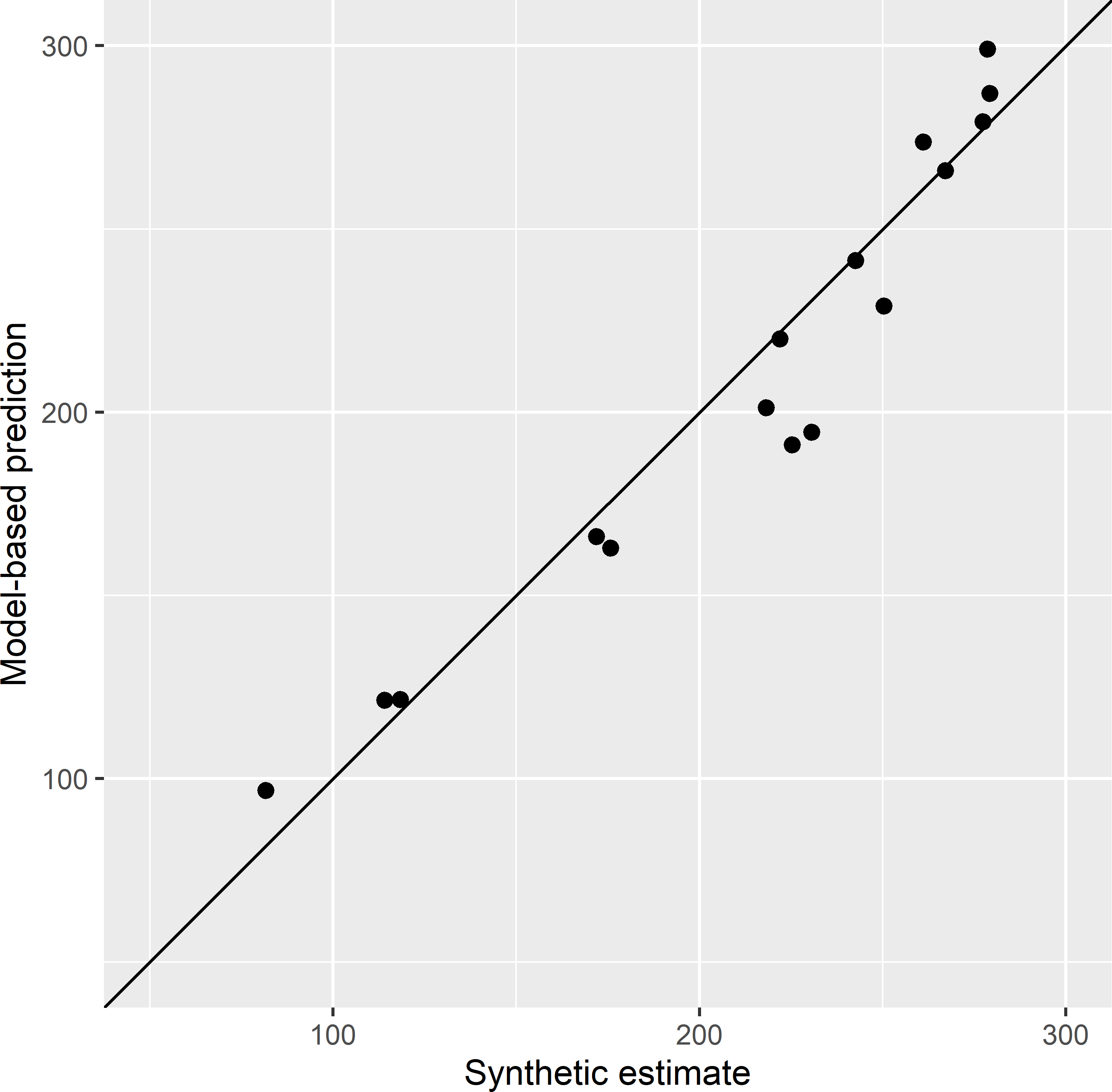
Figure 14.2: Scatter plot of the model-based prediction and the synthetic estimate of the mean AGB (109 kg ha-1) of ecoregions in Eastern Amazonia. The solid line is the 1:1 line.
The most striking difference is the standard error. The standard errors of the synthetic estimator range from 3.7 to 7.1 (Table 14.6), whereas the standard errors of the geostatistical predictions range from 5.9 to 15.9. However, these two standard errors are fundamentally different and should not be compared. The standard error of the synthetic estimator is a sampling standard error, i.e., it quantifies the variation of the estimated mean of an ecoregion over repeated random sampling with the sampling design, in this case simple random sampling of 200 units. The model-based standard error is not a sampling standard error but a model standard error, which expresses our uncertainty about the means of the domains due to our imperfect knowledge of the spatial variation of AGB. Given the observations of AGB at the selected sample, the map with the covariate lnSWIR2, and the estimated semivariogram model parameters, we are uncertain about the exact value of AGB at unsampled units. No samples are considered other than the one actually selected. For the fundamental difference between design-based, model-assisted, and model-based estimates of means, refer to Section 1.2 and Chapter 26.
It makes more sense to compare the two model-based predictions, the random intercept model predictions and the geostatistical predictions, and their standard errors. Figure 14.3 shows that the two model-based predictions are very similar.
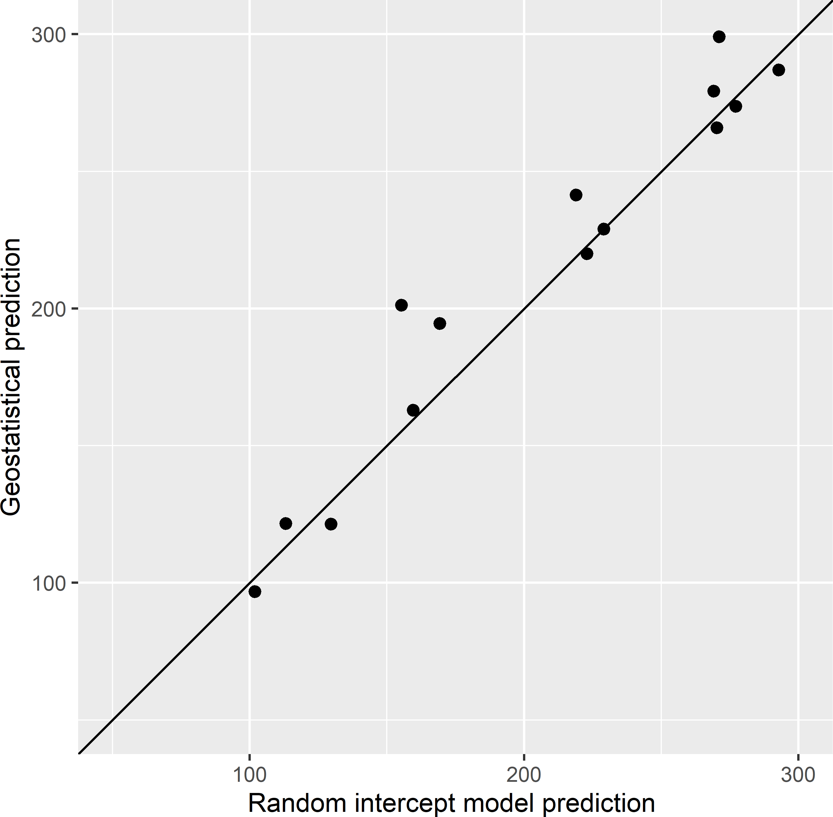
Figure 14.3: Scatter plot of model-based predictions of the mean AGB (109 kg ha-1) of ecoregions in Eastern Amazonia, obtained with the random intercept model and the geostatistical model. The solid line is the 1:1 line.
For six ecoregions, the standard errors of the geostatistical model predictions are much smaller than those of the random intercept model predictions (Figure 14.4). These are ecoregions with small sample sizes.
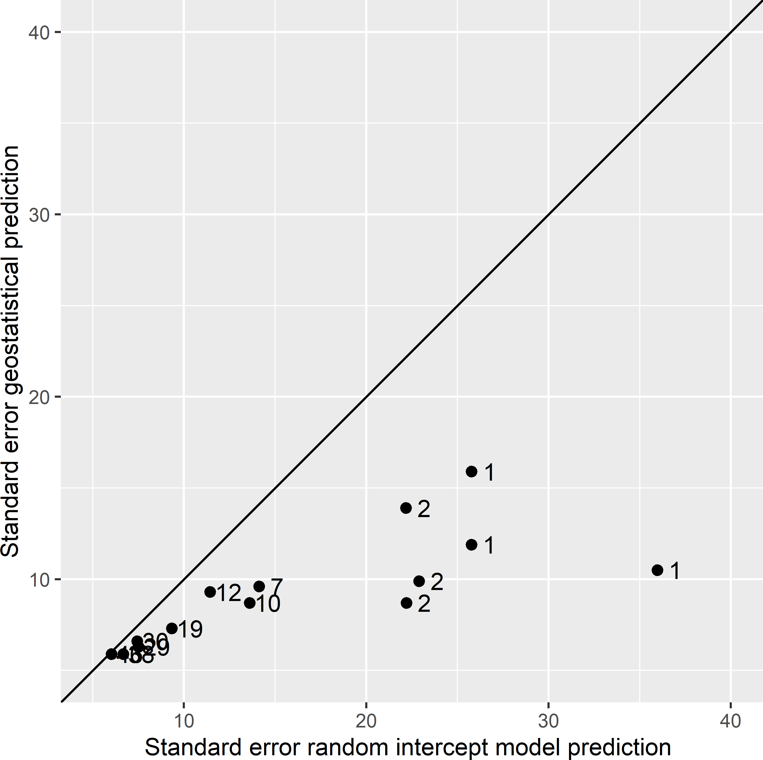
Figure 14.4: Scatter plot of the estimated standard error of model-based predictions of the mean AGB (109 kg ha-1) of ecoregions obtained with the random intercept model and the geostatistical model, using a simple random sample without replacement of size 200 from Eastern Amazonia. The numbers refer to the number of sampling units in an ecoregion. The solid line is the 1:1 line.
14.4 Supplemental probability sampling of small domains
The sample size in small domains of interest can be so small that no reliable statistical estimate of the mean or total of these domains can be obtained. In this case, we may decide to collect a supplemental sample from these domains. It is convenient to use these domains as strata in supplemental probability sampling, so that we can control the sample sizes in the strata. If we can safely assume that the study variable at the units of the first sample are not changed, there is no need to revisit these units; otherwise, we must revisit them to observe the current values.
There are two approaches for using the two probability samples to estimate the population mean or total of a small domain (Grafström et al. 2019). In the first approach, the two samples are combined, and then the merged sample is used to estimate the population mean or total. In the second approach, the samples are not combined, but the two estimates from the separate samples. In this section only the first approach is illustrated with a simple situation in which the two samples are easily combined. Refer to Grafström et al. (2019) for a more general approach of how multiple probability samples can be combined.
Suppose that the original sample is a simple random sample from the entire study area. A supplemental sample is selected from small domains, i.e., domains that have few selected units only. For a given small domain, the first sample is supplemented by selecting a simple random sample from the units not yet selected in the first sample. The size of the supplemental sample of a domain depends on the number of units of that domain in the first sample. The first sample is supplemented so that the total sample size of that domain is fixed. In this case, the combined sample of a domain is a simple random sample from that domain, so that the usual estimators for simple random sampling can be used to estimate the domain mean or total and its standard error.
This sampling strategy is illustrated with Eastern Amazonia. A simple random sample without replacement of 400 units is selected.
grdAmazonia$Biome <- as.factor(grdAmazonia$Biome)
biomes <- c("Mangrove", "Forest_dry", "Grassland", "Forest_moist")
levels(grdAmazonia$Biome) <- biomes
n1 <- 400
set.seed(123)
units_1 <- sample(nrow(grdAmazonia), size = n1, replace = FALSE)
mysample_1 <- grdAmazonia[units_1, c("AGB", "Biome")]
print(n1_biome <- table(mysample_1$Biome))
    Mangrove   Forest_dry    Grassland Forest_moist
           2            9           26          363
The selected units are removed from the sampling frame. For each of the three small biomes, Mangrove, Forest_dry, and Grassland, the size of the supplemental sample is computed so that the total sample size becomes 40. The supplemental sample is selected by stratified simple random sampling without replacement, using the small biomes as strata (Chapter 4).
units_notselected <- grdAmazonia[-units_1, ]
Biomes_NFM <- units_notselected[units_notselected$Biome != "Forest_moist", ]
n_biome <- 40
n2_biome <- rep(n_biome, 3) - n1_biome[-4]
ord <- unique(Biomes_NFM$Biome)
units_2 <- sampling::strata(Biomes_NFM, stratanames = "Biome",
  size = n2_biome[ord], method = "srswor")
mysample_2 <- getdata(Biomes_NFM, units_2)
mysample_2 <- mysample_2[c("AGB", "Biome")]
The two samples are merged, and the means of the domains are estimated by the sample means.
mysample <- rbind(mysample_1, mysample_2)
print(mz_biome <- tapply(mysample$AGB, INDEX = mysample$Biome, FUN = mean))
Mangrove Forest_dry Grassland Forest_moist
112.8000 122.1750 123.6250 233.6749 Finally, the standard error is estimated, accounting for sampling without replacement from a finite population (Equation (3.11)).
N_biome <- table(grdAmazonia$Biome)
fpc <- (1 - n_biome / N_biome)
S2z_biome <- tapply(mysample$AGB, INDEX = mysample$Biome, FUN = var)
print(se_mz_biome <- sqrt(fpc * (S2z_biome / n_biome)))
    Mangrove   Forest_dry    Grassland Forest_moist
    5.227434     8.213407    11.709257    13.937597
This sampling approach and estimation are repeated 10,000 times, i.e., a simple random sample without replacement of size 400 is selected 10,000 times from Eastern Amazonia, and the samples from the three small domains are supplemented so that the total sample sizes in these domains become 40. In two out of the 10,000 samples, the size of the first sample in one of the domains exceeded 40 units. These two samples are discarded. Ideally, these samples are not discarded, but their sizes in the small domains are reduced to 40 units, which are then used to estimate the means of the domains.
| Mangrove | Dry forest | Grassland | |
|---|---|---|---|
| Average of estimated means | 122.476 | 113.983 | 114.462 |
| True means | 122.494 | 113.931 | 114.390 |
| Standard deviation of estimated means | 6.186 | 7.563 | 10.986 |
| Average of estimated standard errors | 6.169 | 7.450 | 10.946 |
| Coverage rate 95% | 0.950 | 0.937 | 0.945 |
| Coverage rate 90% | 0.903 | 0.888 | 0.896 |
| Coverage rate 80% | 0.801 | 0.792 | 0.799 |
For all three small domains, the average of the 10,000 estimated means of AGB is about equal to the true mean (Table 14.9). Also the mean of the 10,000 estimated standard errors is very close to the standard deviation of the 10,000 estimated means. The coverage rates of 95, 90, and 80% confidence intervals are about equal to the nominal coverage rates.
This simple approach is feasible because at the domain level the two merged samples are a simple random sample. This approach is also applicable when the first sample is a stratified simple random sample from the entire population, and the supplemental sample is a stratified simple random sample from a small domain using as strata the intersections of the strata used in the first phase and that domain.