A Answers to exercises

R scripts of the answers to the exercises are available in the Exercises folder at the github repository of this book.

Introduction to probability sampling

1. No, this is not a probability sample because, with this implementation, the probabilities of selection of the units are unknown.
   
2. For simple random sampling without replacement, the inclusion probability is 0.5 (\(\pi_k= n/N = 2/4\)). For simple random sampling with replacement, the inclusion probability is 0.4375 (\(\pi_k = 1- (1-1/N)^n = 1-0.75^2\)).

Simple random sampling

1. The most remarkable difference is the much smaller range of values in the sampling distribution of the estimator of the population mean (Figure 3.2). This can be explained by the smaller variance of the average of \(n\) randomly selected values compared to the variance of an individual randomly selected value. A second difference is that the sampling distribution is more symmetric, less skewed to the right. This is an illustration of the central limit theorem.
   
2. The variance (and so the standard deviation) becomes smaller.
   
3. Then the difference between the average of the estimated population means and the true population mean will be very close to 0, showing that the estimator is unbiased.
   
4. For simple random sampling without replacement (from a finite population), the sampling variance will be smaller. When units are selected with replacement, a unit can be selected more than once. This is inefficient, as there is no extra information in the unit that has been selected before.
   
5. The larger the population size \(N\), the smaller the difference between the sampling variances of the estimator of the mean for simple random sampling with replacement and simple random sampling without replacement (given a sample size \(n\)).
   
6. The true sampling variance of the estimator of the mean for simple random sampling from an infinite population can be computed with the population variance divided by the sample size: \(V(\hat{\bar{z}})=S^2(z)/n\).
   
7. In reality, we cannot compute the true sampling variance, because we do not know the values of \(z\) for all units in the population, so that we do not know the population variance \(S^2(z)\).
   
8. See SI.R. The 90% confidence interval is less wide than the 95% interval, because a larger proportion of samples is allowed not to cover the population mean. The estimated standard error of the estimated total underestimates the true standard error, because a constant bulk density is used. In reality this bulk density also varies.

Stratified simple random sampling

1. See STSI1.R.
   
2. Strata EA and PA can be merged without losing much precision: their means are about equal.
   
3. See STSI2.R. The true sampling variance of the \(\pi\) estimator of the mean SOM obtained by collapsing strata EA and PA equals 42.89, whereas the sampling variance with the original stratification equals 42.53. So, the new stratification with four strata is only slightly worse.
   
4. The proof is as follows: \(\sum_N \pi_k=\sum_H \sum_{N_h}\pi_{hk}=\sum_H \sum_{N_h}n_h/N_h=\sum_H n_h=n\).
   
5. See STSIcumrootf.R. The default allocation is Neyman allocation, see help of function strata.cumrootf. The true sampling variance of the estimator of the mean equals 20.0. The stratification effect equals 4.26.
   
6. With at least two points per geostratum, the variance of the estimator of the stratum mean can be estimated without bias by the estimated stratum variance divided by the number of points in that stratum. However, despite the absence of bias, the estimator of the variance of the population mean can be quite inaccurate (large mean squared error). For that reason one may prefer to select one point per geostratum. The variance of the population total can then be estimated by Equation (9.9).
   
7. On average, the sampling variance of the estimator of the mean with 100 \(\times\) 1 point is smaller than with \(50 \times 2\) points, because the geographical spreading will be somewhat better (less spatial clustering).
   
8. With geostrata of equal size and equal number of sampling points per geostratum, the sampling intensity is equal for all strata, so that the sample mean is an unbiased estimator of the population mean. In formula: \(\hat{\bar{z}}= \sum\limits_{h=1}^{H} w_{h}\,\bar{z}_{\mathcal{S}h} = \frac{1}{H} \sum\limits_{h=1}^{H} \bar{z}_{\mathcal{S}h} = \bar{z}_{\mathcal{S}}\), with \(\bar{z}_{\mathcal{S}h}\) the average of the sample from stratum \(h\) and \(\bar{z}_{\mathcal{S}}\) the average of all sampling points.
   
9. See STSIgeostrata.R.
   • Collapsing the geostrata on the basis of the measurements of the study variable is not a proper way, as it will lead to a biased estimator of the sampling variance of the estimator of the mean. The estimated stratum variances \(\widehat{S}^2(z)\) will be small, and so the estimated sampling variance will underestimate the true sampling variance.
   • I propose to group neighbouring geostrata, i.e., geostrata that are close to each other.
   • The sampling variance estimator is not unbiased. The sampling variance is slightly overestimated, because we assume that the two (or three) points within a collapsed stratum are selected by simple random sampling, whereas they are selected by stratified random sampling (a collapsed stratum consists of two or three geostrata), and so there is less spatial clustering compared to simple random sampling.
     
10. See STSIgeostrata_composite.R.
    • No, with bulking within strata the sampling variance cannot be estimated, because then we cannot estimate the sampling variances of the estimated stratum means, which are needed for estimating the sampling variance of the estimator of the population mean.
    • If all aliquots are analysed separately, the estimated population mean is more precise than with composite sampling (variance of the estimator of the mean is smaller), because the contribution of the measurement error to the total variance of the estimator of the mean is smaller.
    • This combination of arguments of function stratify does not work, because with geostrata of unequal area the mean of a composite sample is a biased estimator of the population mean. All aliquots bulked into a composite get equal weight, but they should get different weights, because they do not represent equal fractions of the population.

Systematic random sampling

1. See SY.R.
   
2. As can be seen in the plot, the spatial coverage of the study area by the two systematic random samples can be quite poor. So, I expect that the variance of the estimator of the mean using the data of two systematic random samples of half the expected size is larger than the variance of the estimator of the mean based on the data of a single systematic random sample.

Cluster random sampling

1. See Cluster.R.
   
2. I expect that the sampling variance with three transects is larger than with six transects of half the length, as the sampling points are more spatially clustered.
   
3. With two independently selected clusters per stratum, the sampling variance of the estimator of the mean can be estimated without bias, as the variance of cluster means within the strata can be estimated from the two cluster means.

Two-stage cluster random sampling

1. See TwoStage.R.
   

2. With ten PSU draws and four SSUs per PSU draw (10 \(\times\) 4), the expected standard error of the estimator of the population mean is smaller than with four PSU draws and ten SSUs per PSU draw (\(4 \times 10\)), because spatial clustering of the sampling points is less strong.
   

3. See TwoStage.R.
   

4. See TwoStage.R.
   

5. See TwoStage.R.
   

6. For the first variance component: \[\begin{equation} \begin{split} \frac{1}{n} \sum_{j=1}^N p_j\left(\frac{t_j(z)}{p_j}-t(z)\right)^2 = \frac{1}{n} \sum_{j=1}^N p_j\left(M\frac{t_j(z)}{M_j}-M\bar{z}\right)^2 \\ = \frac{1}{n} \sum_{j=1}^N p_j\left(M\left(\bar{z}_j-\bar{z}\right)\right)^2 = \frac{M^2}{n} \sum_{j=1}^N p_j\left(\bar{z}_j-\bar{z}\right)^2 \;. \end{split} \end{equation}\]

   For the second variance component: \[\begin{equation} \begin{split} \frac{1}{n} \sum_{j=1}^N \frac{M_j^2 S^2_j}{m_j p_j} =\frac{1}{nm} \sum_{j=1}^N \frac{M_j^2 S^2_j}{p_j} = \frac{1}{nm} \sum_{j=1}^N M M_j S^2_j \\ =\frac{1}{nm} \sum_{j=1}^N M^2 \frac{M_j}{M} S^2_j =\frac{M^2}{nm} \sum_{j=1}^N p_j S^2_j \;. \end{split} \end{equation}\]

   Division of both variance components by \(M^2\) yields the variance of the estimator of the population mean, see Equations (7.3), (7.4), and (7.5).

Sampling with probabilities proportional to size

1. See pps.R.
   
2. No, this field should not be included in the poppy area of that sampling unit, because it is located outside the target area.
   
3. Yes, this field must be included in the poppy area of that sampling unit, as it is located inside the target area. The target area is the territory of Kandahar, regardless of how an area inside this territory is depicted on the map, as agricultural land or otherwise.

Balanced and well-spread sampling

1. See Balanced.R.
   
2. Spatial clustering of sampling units with balanced sampling may lead to a less precise estimate of the population mean. This will be the case when the residuals of the regression model are spatially correlated (show spatial structure). The residuals will be correlated when the spatial variation of the study variable is also determined by covariates or factors that are not used in balancing the sample. If the residuals are not spatially correlated (white noise), spatial clustering does no harm.
   
3. One advantage is that unequal inclusion probabilities can be used in the LPM design. If the sampling units have unequal size (as in the poppy survey of Kandahar), or if a covariate is available that is linearly related to the study variable (as in the AGB survey of Eastern Amazonia), the sampling efficiency can be increased by sampling with (inclusion) probabilities proportional to size. The only option for random sampling from geostrata is then to select the units within geostrata by pps sampling.

Model-assisted estimation

1. See RegressionEstimator.R. The approximate standard error estimator that uses the \(g\)-weights (computed with functions calibrate and svymean of package survey) has a larger mean (7.194) than the approximated standard error (7.130) computed with Equation (10.13).
   

2. See VarianceRegressionEstimator.R. In reality, we do not have a population fit of the regression coefficients, but these coefficients must be estimated from a sample. The estimated coefficients vary among the samples, which explains that the experimental variance, i.e., the variance of the 10,000 regression estimates obtained by estimating the coefficients from the sample (Sample in Figure A.1), is larger than the variance as computed with the population fit of the regression coefficients (Exhaust in Figure A.1).

   The difference between the experimental variance (variance of regression estimator with sample fit of coefficients) and the variance obtained with the population fit, as a proportion of the experimental variance, decreases with the sample size. The same holds for the difference between the approximated variance and the experimental variance as a proportion of the experimental variance. Both findings can be explained by the smaller contribution of the variance of the estimated regression coefficients to the variance of the regression estimator with the large sample size. The approximated variance does not account for the uncertainty about the regression coefficients, so that for all three sample sizes this approximated variance is about equal to the variance of the regression estimator as computed with the population fit of the regression coefficients.

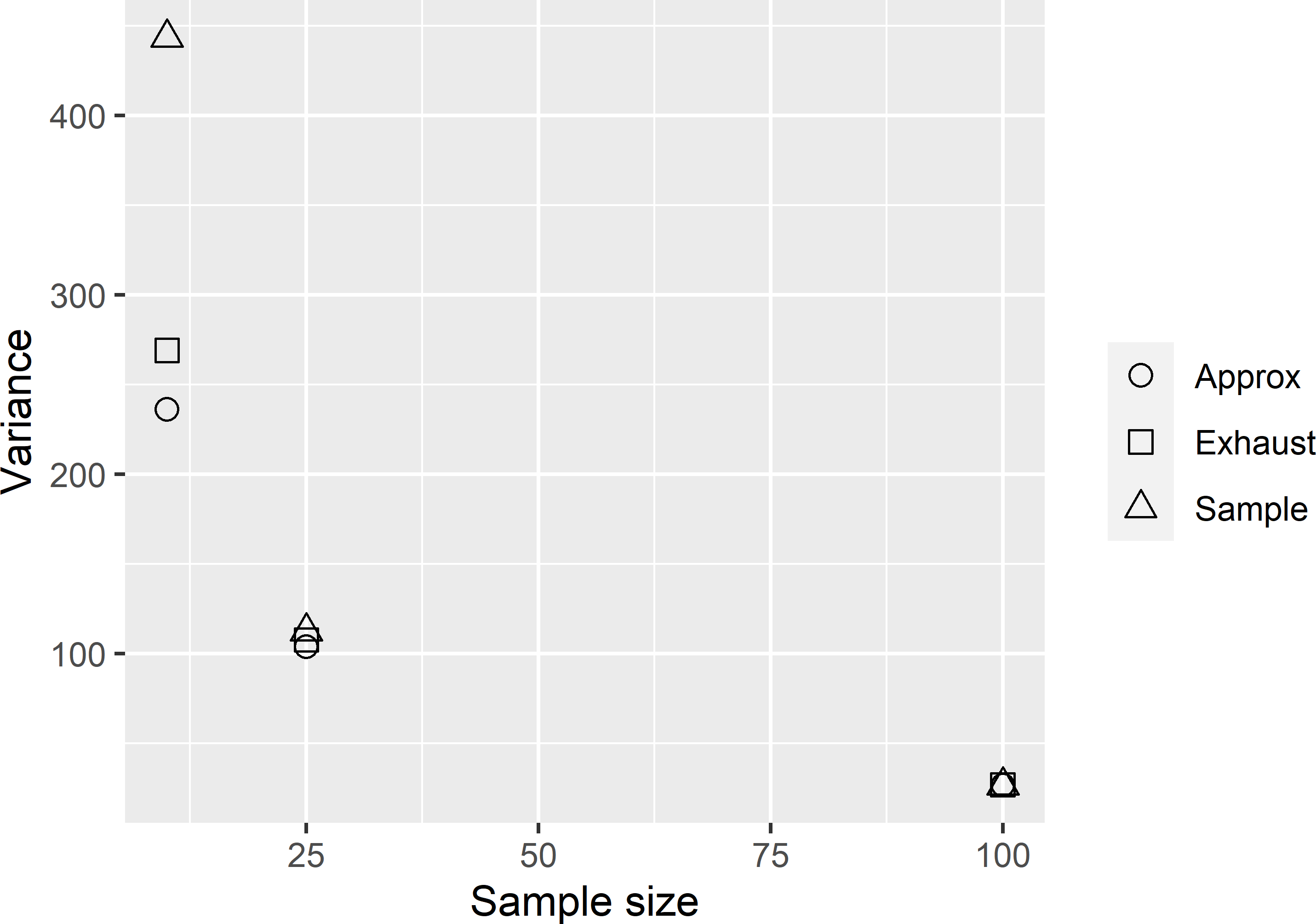
Figure A.1: Variance of the regression estimator of the mean AGB in Eastern Amazonia with population fit of regression coefficients (Exhaust), with sample fit of regression coefficients (Sample), and approximated variance of regression estimator (Approx).

3. See RatioEstimator.R. The population fit of the slope coefficient of the homoscedastic model differs from the ratio of the population total poppy area to the population total agricultural area. For the heteroscedastic model, these are equal.

Two-phase random sampling

1. See RegressionEstimator_Twophase.R. Figure A.2 shows the approximated sampling distribution of the simple regression estimator of the mean AGB in Eastern Amazonia when lnSWIR2 is observed for all sampling units (one-phase), and when AGB is observed for the subsample only (two-phase). The variance of the regression estimator with two-phase sampling is considerably larger. Without subsampling, the regression estimator exploits our knowledge of the population mean of the covariate lnSWIR2, whereas in two-phase sampling, this population mean must be estimated from the first-phase sample, introducing additional uncertainty.

   The average of the 10,000 approximated variances equals 40.5 (10⁹ kg ha^-1)², which is considerably smaller than the variance of the 10,000 regression estimates for two-phase sampling, which is equal to 51.2 (10⁹ kg ha^-1)².

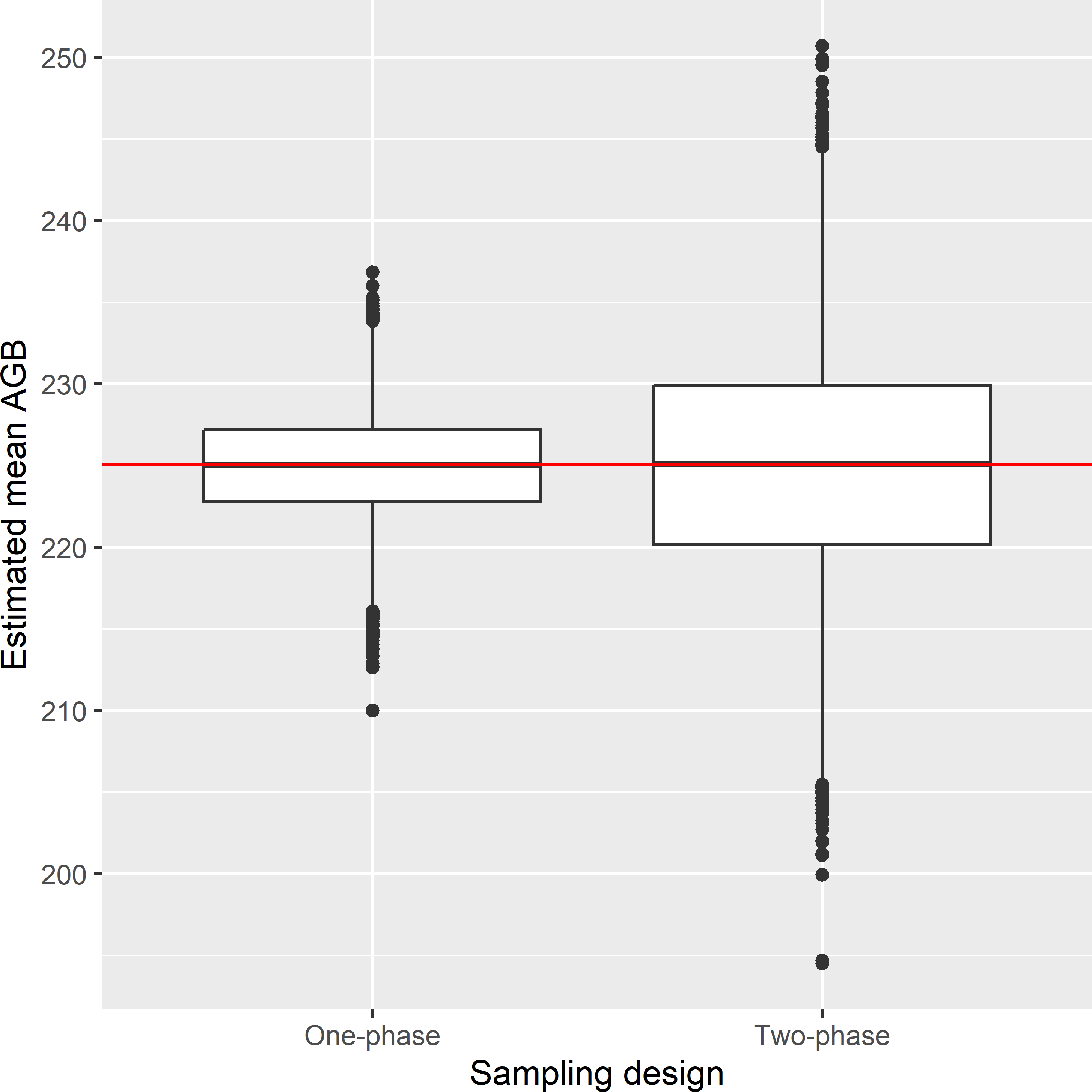
Figure A.2: Approximated sampling distribution of the simple regression estimator of the mean AGB (10⁹ kg ha^-1) in Eastern Amazonia in the case that the covariate is observed for all sampling units (one-phase) and for the subsample only (two-phase).

Computing the required sample size

1. See RequiredSampleSize_CIprop.R. Figure A.3 shows that the required sample size decreases sharply with the length of the confidence interval and increases with the prior (anticipated) proportion.

   A prior for the proportion is needed because the standard error of the estimated proportion is a function of the estimated proportion \(\hat{p}\) itself: \(se(\hat{p})=\frac{\sqrt{\hat{p}(1-\hat{p})}}{\sqrt{n}}\), so that the length of the confidence interval, computed with the normal approximation, is also a function of \(\hat{p}\), see Equation (12.11).

   For a prior proportion \(p^*\) of 0.5 the standard deviation \(\sqrt{p^*(1-p^*)}\) is maximum. The closer the prior proportion to zero or one, the smaller the standard error of the estimated proportion, the smaller the required sample size.

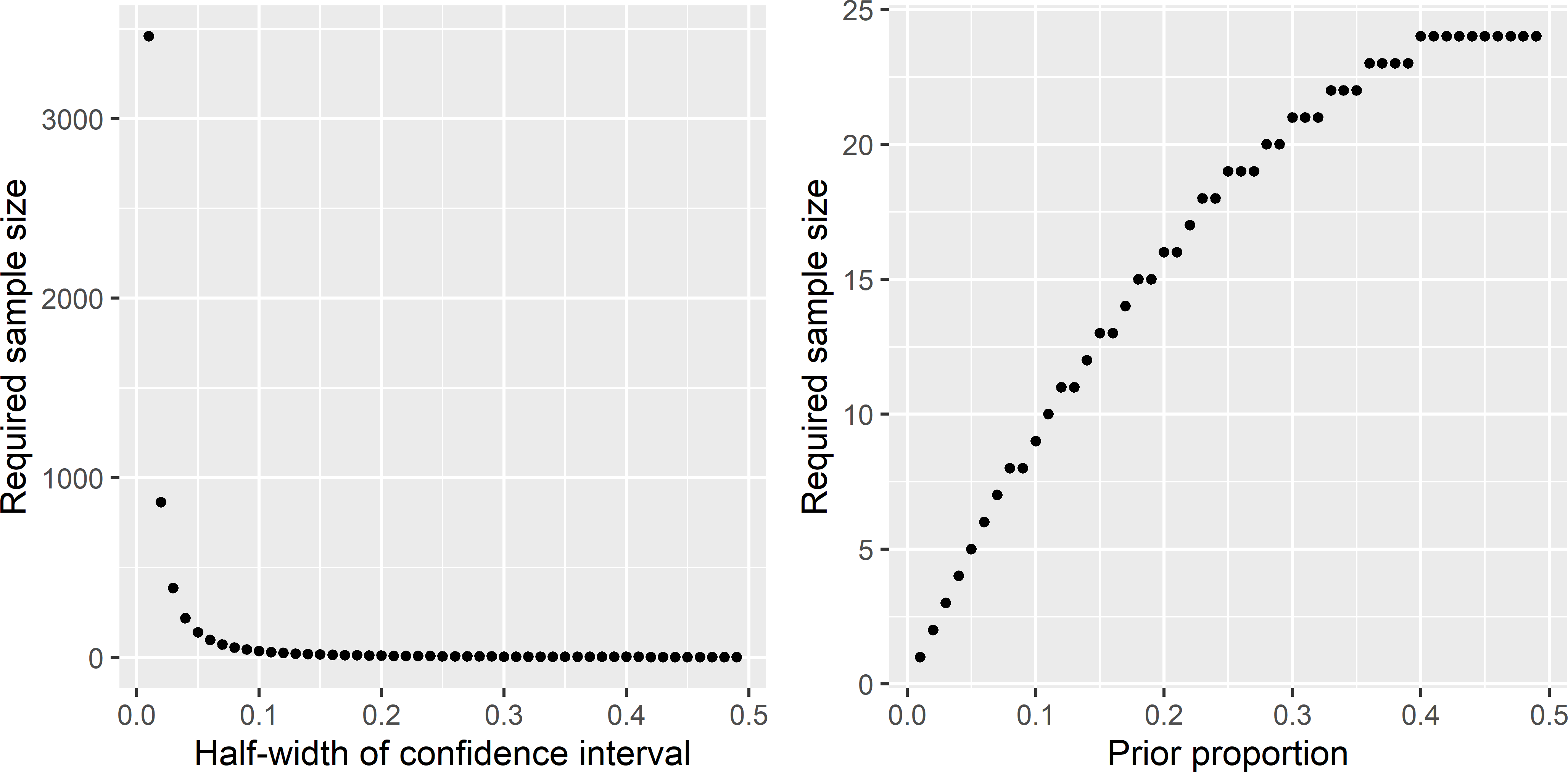
Figure A.3: Required sample size as a function of the half-length of a 95% confidence interval of the population proportion, for a prior proportion of 0.1 (left subfigure), and as a function of the prior proportion for a half-length of a 95% confidence interval of 0.2 (right subfigure).

2. See RequiredSampleSize_CIprop.R. There is no need to compute the required sample size for prior proportions \(>0.5\), as this required sample size is symmetric. For instance, the required sample size for \(p^*=0.7\) is equal to the required sample size for \(p^*=0.3\).

Model-based optimisation of probability sampling designs

1. See MBSamplingVarSI_VariogramwithNugget.R. The predicted sampling variance is slightly larger compared to the predicted sampling variance obtained with the semivariogram without nugget (and the same sill and range), because 50% of the spatial variation is not spatially structured, so that the model-expectation of the population variance (the predicted population variance) is larger.
   
2. See first part of MBRequiredSampleSize_SIandSY.R.
   
3. See second part of MBRequiredSampleSize_SIandSY.R. The model-based prediction of the required sample size for simple random sampling is 34 and for systematic random sampling 13. The design effect at a sample size of 34 equals 0.185. The design effect decreases with the sample size, i.e., the ratio of the variance with systematic random sampling to the variance with simple random sampling becomes smaller. This is because the larger the sample size, the more we profit from the spatial correlation.

Repeated sample surveys for monitoring population parameters

1. See SE_STparameters.R. For the designs SP and RP, the true standard errors of all space-time parameters are slightly smaller than the standard deviations in Table 15.1, because in the sampling experiment the estimated covariances of the elementary estimates are used in the GLS estimator of the spatial means, whereas in this exercise the true covariances are used. The estimated covariances vary among the space-time samples. This variation propagates to the GLS estimates of the spatial means and so to the estimated space-time parameters.
   
2. See SE_ChangeofMean_HT.R. The standard error of the change with the GLS estimators of the two spatial means is much smaller than the standard error of the change with the \(\pi\) estimators, because the GLS estimators use the data of all four years to estimate the spatial means of 2004 and 2019, whereas with the \(\pi\) estimators only the data of 2004 and 2019 are used.

Regular grid and spatial coverage sampling

1. See SquareGrid.R. The number of grid points specified with argument n is the expected number of grid points over repeated selection of square grids with a random start. With a fixed start (using argument offset), the number of grid points can differ from the expected sample size.
   
2. The optimal spatial coverage sample, optimal in terms of MSSD, consists of the four points in the centre of the four subsquares of equal size.
   
3. If we are also interested in the accuracy of the estimated plot means, the sampling units can best be selected by probability sampling, for instance by simple random sampling, from the subsquares, or strata. Preferably at least two points should then be selected from the strata, see Section 4.6.
   
4. See SpatialCoverageCircularPlot.R. See Figure A.4.

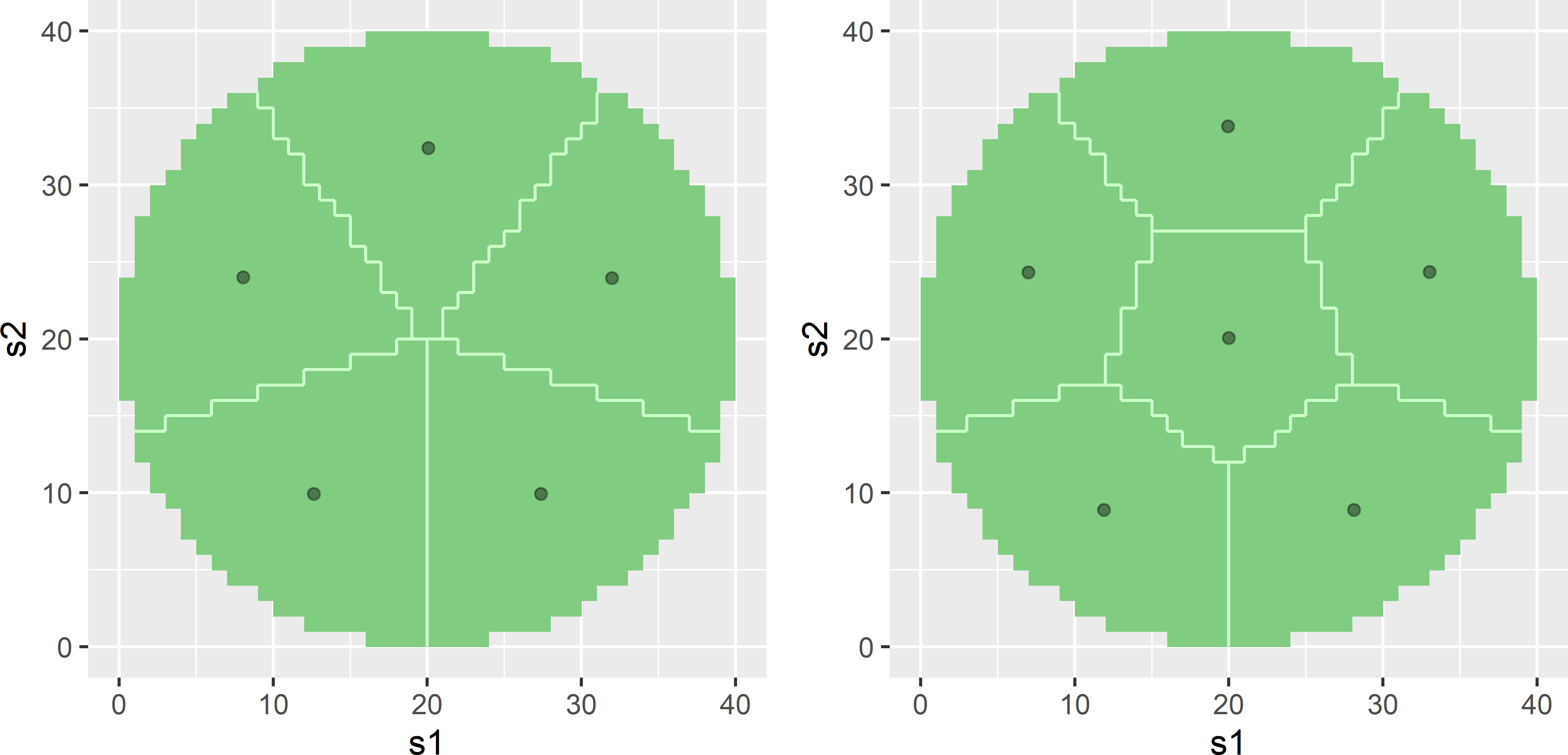
Figure A.4: Spatial coverage samples of five and six points in a circular plot.

5. Bias can be avoided by constructing strata of equal size. Note that in this case we cannot use function spsample to select the centres of these geostrata. These centres must be computed by hand.
   
6. See SpatialInfill.R.

Covariate space coverage sampling

1. See CovariateSpaceCoverageSample.R. See Figure A.5.

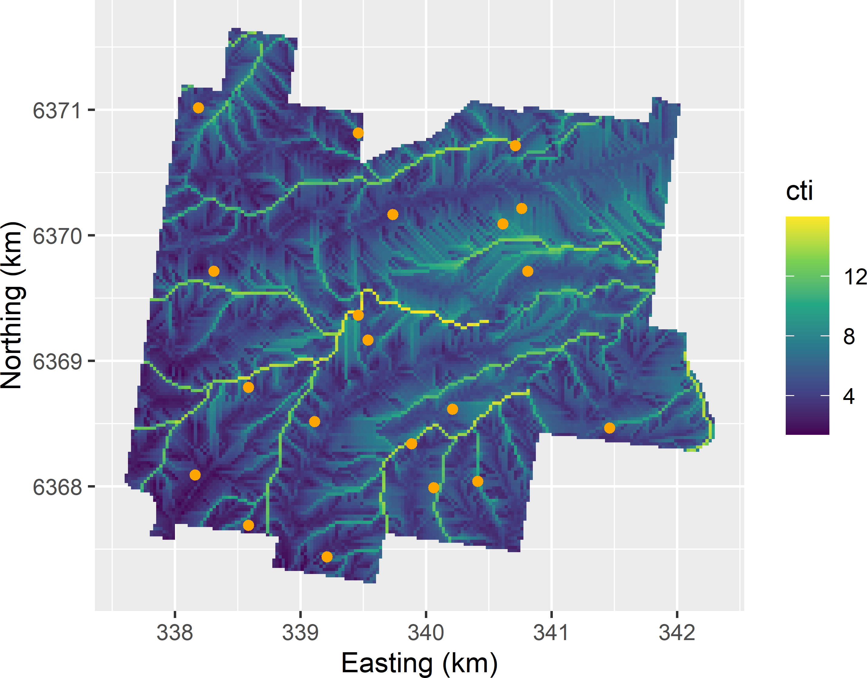
Figure A.5: Covariate space coverage sample from Hunter Valley, using cti, ndvi, and elevation as clustering variables, plotted on a map of cti.

Conditioned Latin hypercube sampling

1. See cLHS.R. Most units are selected in the part of the diagram with the highest density of raster cells. Raster cells with a large cti value and low elevation and raster cells with high elevation and small cti value are (nearly) absent in the sample. In the population, not many raster cells are present with these combinations of covariate values.
   
2. See cLHS_Square.R.
   • Spatial coverage is improved by using the spatial coordinates as covariates, but it is not optimal in terms of MSSD.
   • It may happen that not all marginal strata of \(s1\) and \(s2\) are sampled. Even when all these marginal strata are sampled, this does not guarantee a perfect spatial coverage.
   • With set.seed(314) and default values for the arguments of function clhs, there is one unsampled marginal stratum and one marginal stratum with two sampling locations. So, component O1 equals 2. The minimised value (2.62) is slightly larger due to the contribution of O3 to the criterion.

Model-based optimisation of the grid spacing

1. See MBGridspacing_QOKV.Rmd. For P50 not to exceed 0.85 the tolerable grid spacing is about 11.7 km, for P80 it is 9.4 km, and for P95 it is 7.1 km (Figure A.6).

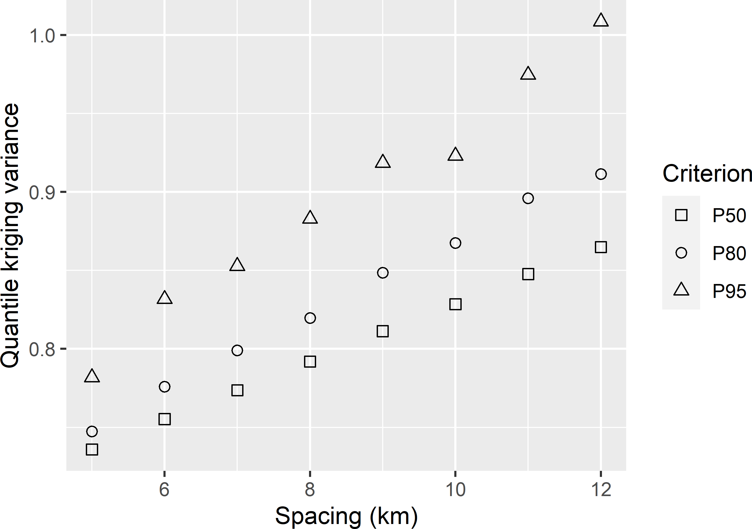
Figure A.6: Three quantiles of the ordinary kriging variance of predicted SOM concentrations in West-Amhara, as a function of the grid spacing.

2. See MBGridspacing_Sensitivity.Rmd. Increasing the nugget by 5% and decreasing the range by 5% yields a tolerable grid spacing that is smaller than that with the original semivariogram (Figure A.7). The tolerable grid spacings for a mean kriging variance of 0.85 are 10.6, 8.9, and 7.4 km for the original semivariogram, the semivariogram with increased nugget, and the semivariogram with the smaller range, respectively, leading to a required expected sample size of 97, 137, and 200 points.

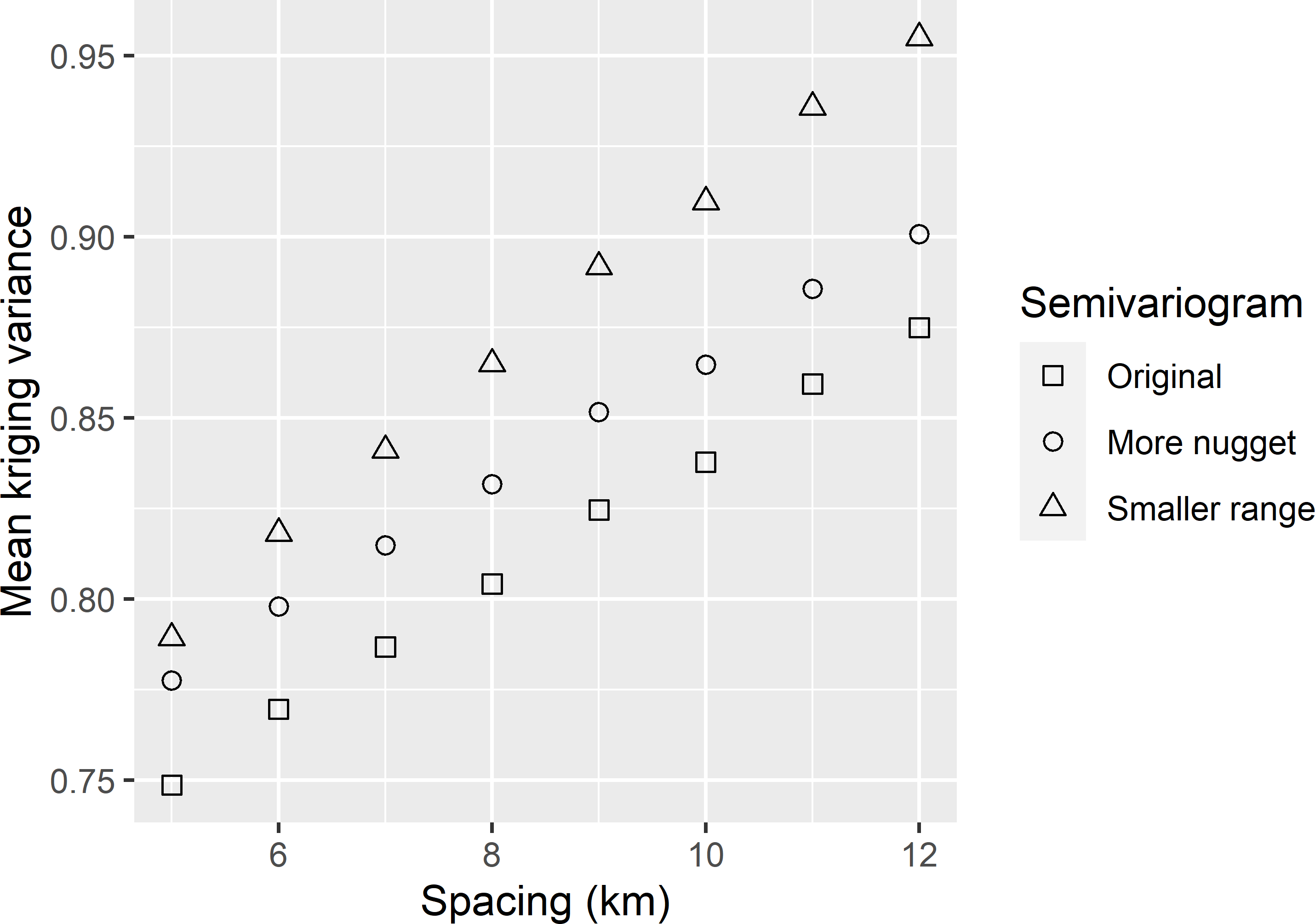
Figure A.7: Mean ordinary kriging variance of predicted SOM concentrations in West-Amhara, as a function of grid spacing for three semivariograms.

3. The variation in MKV for a given grid spacing can be explained by the random sample size: for a given spacing, the number of points of a randomly selected grid inside the study area is not fixed but varies. Besides, the covariate values at the grid points vary, so that also the variance of the estimator of the mean, which contributes to the kriging variance, differs among grid samples.
   
4. See MBGridspacing_MKEDV.Rmd. The tolerable grid spacing for a mean kriging variance of 0.165 is 79 m.

Model-based optimisation of the sampling pattern

1. See MBSampleSquare_OK.Rmd. The optimised sample (Figure A.8) is most likely not the global optimum. The spatial pattern is somewhat irregular. I expect the optimal sampling locations to be close to the centres of the subsquares.

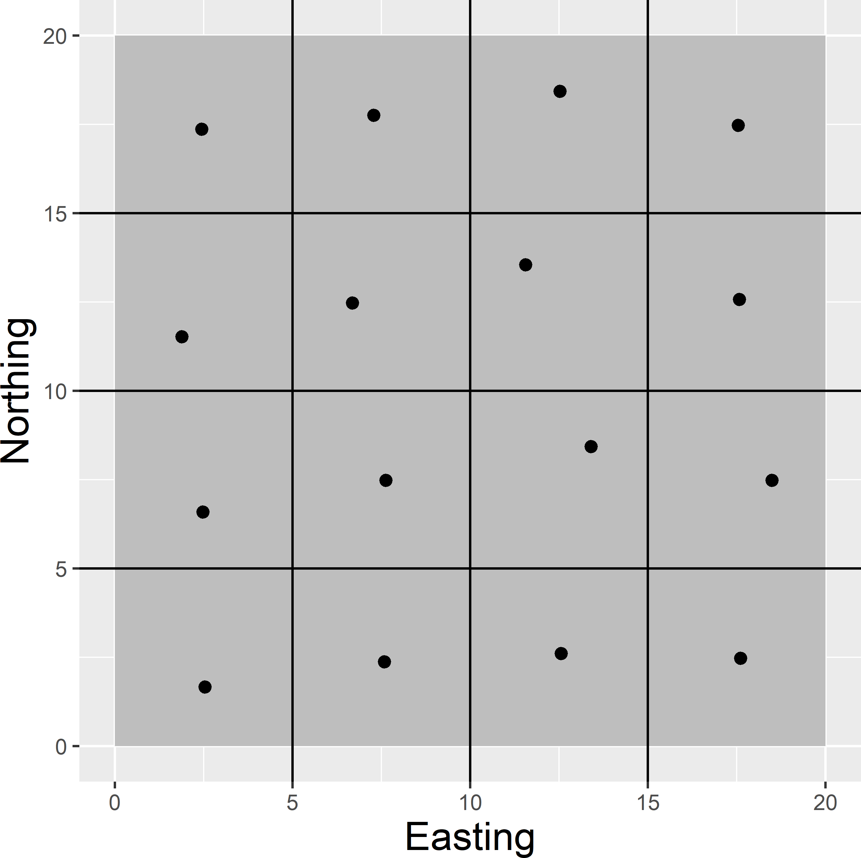
Figure A.8: Optimised sampling pattern of 16 points in a square for ordinary kriging.

2. See MBSample_QOKV.Rmd. Figure A.9 shows the optimised sampling pattern. Compared with the optimised sampling pattern using the mean ordinary kriging variance (MOKV) as a minimisation criterion (Figure 23.3), the sampling locations are pushed more to the border of the study area. This is because with a sample optimised for MOKV (and a spatial coverage sample) near the border the kriging variances are the largest. By pushing sampling locations towards the border, the kriging variances in this border zone are strongly reduced.

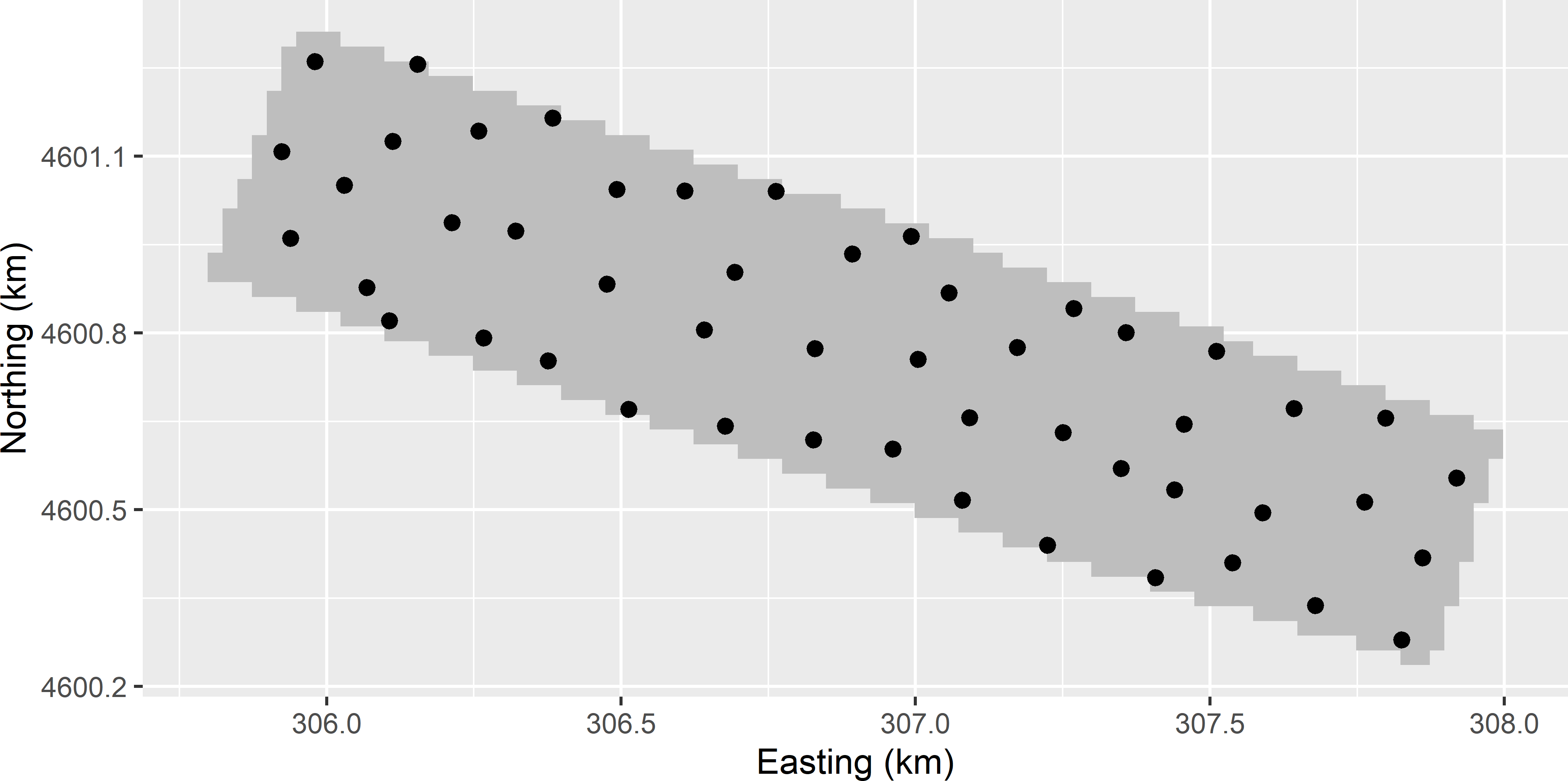
Figure A.9: Optimised sampling pattern of 50 points on the Cotton Research Farm, using the P90 of ordinary kriging predictions of lnECe as a minimisation criterion.

3. See MBSampleSquare_KED.Rmd. Figure A.10 shows the optimised sampling patterns with the three semivariograms.
   • With zero nugget and a (partial) sill of 2, the sampling points are well spread throughout the area (subfigure on the left).
   • With a nugget of 1.5 and a partial sill of 0.5, the sampling points are pushed towards the left and right side of the square. With this residual semivariogram, the contribution of the variance of the predictor of the mean (as a proportion) to the total kriging variance is larger than with the previous semivariogram. By shifting the sampling points towards the left and right side of the square this contribution becomes smaller. At the same time the variance of the interpolation error increases as the spatial coverage becomes worse. The optimised sample is the right balance of these two variance components (subfigure in the middle).
   • With a pure nugget semivariogram, all sampling points are at the left and right side of the square. This is because with a pure nugget semivariogram, the variance of the interpolation error is independent of the locations (the variance equals the nugget variance everywhere), while the variance of the predictor of the mean is minimal for this sample (subfigure on the right).

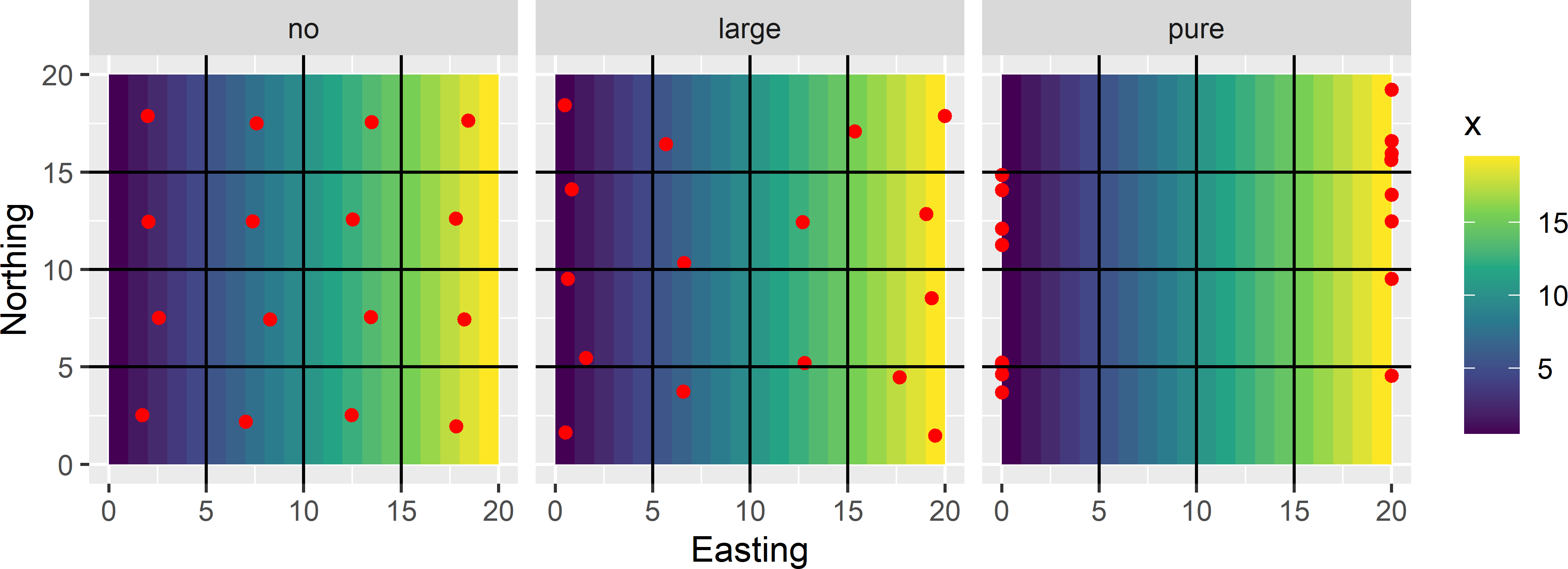
Figure A.10: Effect of the nugget (no nugget, large nugget, pure nugget) on the optimised sampling pattern of 16 points for KED, using Easting as a covariate for the mean.

Sampling for estimating the semivariogram

1. See NestedSampling_v1.R.
   
2. See SI_PointPairs.R. With the seed I used (314), the variance of the estimator of the range parameter with the smaller separation distances is much smaller compared to that obtained with the larger separation distances (the estimated standard error is 115 m).
   
3. See MBSample_SSA_logdet.R. Figure A.11 shows the optimised sampling pattern. The smaller ratio of spatial dependence of 0.5 (larger nugget) results in one cluster of sampling points and many point-pairs with nearly coinciding points.
   
4. See MBSample_SSA_MVKV.R. Figure A.11 shows the optimised sampling pattern. The circular cluster of sampling points covers a larger area than the cluster obtained with a ratio of spatial dependence of 0.8.

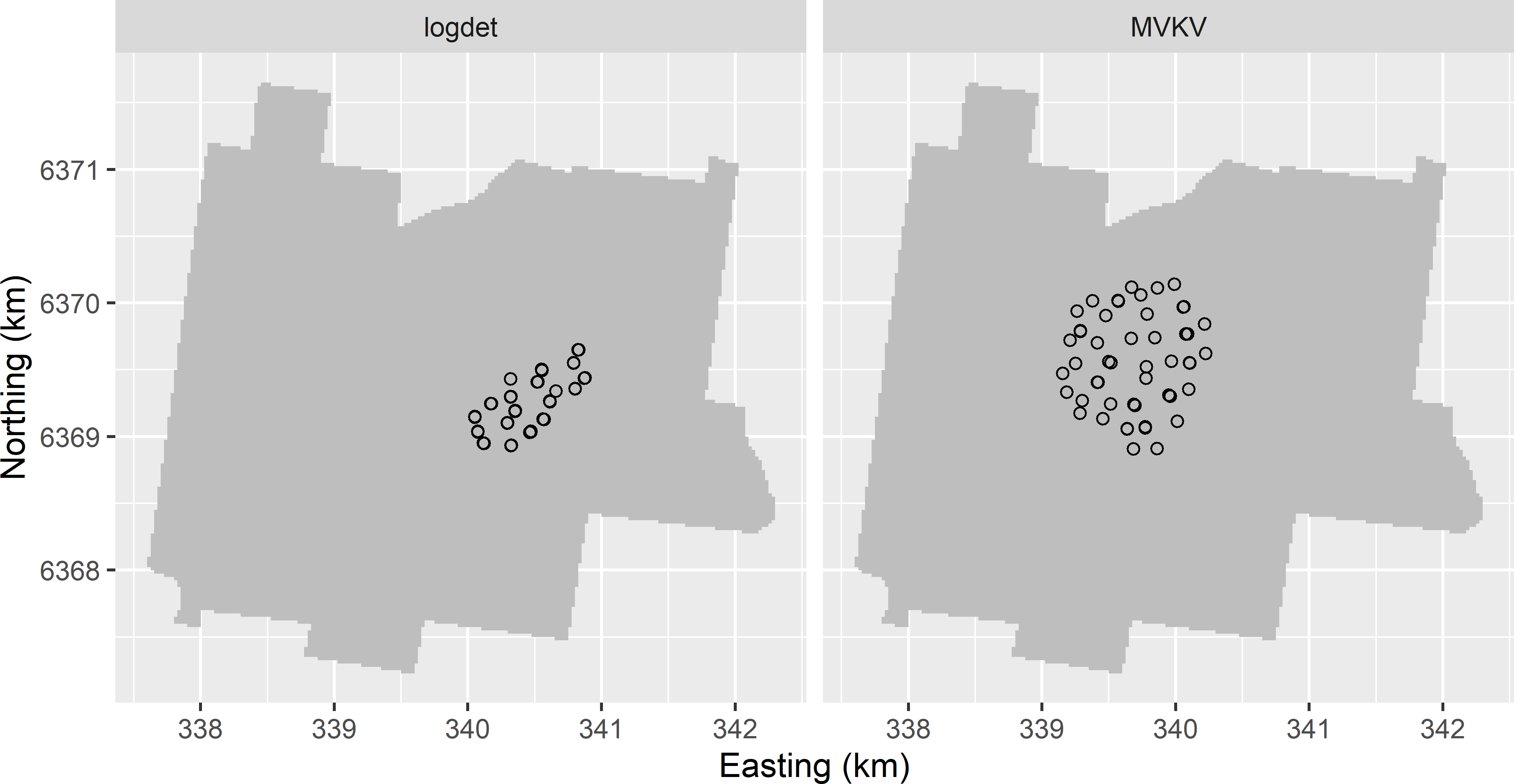
Figure A.11: Model-based sample for estimating the semivariogram, using the log of the determinant of the inverse Fisher information matrix (logdet) and the mean variance of the kriging variance (MVKV) as a minimisation criterion. The sampling pattern is optimised with an exponential semivariogram with a range of 200 m and a ratio of spatial dependence of 0.5.

5. See MBSample_SSA_MEAC.R. Figure A.12 shows the optimised sampling pattern of the 20 sampling points together with the 80 spatial coverage sampling points. The minimised MEAC value equals 0.801, which is slightly smaller than that for the spatial coverage sample of 90 points supplemented by 10 points (0.808).

Figure A.12: Optimised sample of 20 points supplemented to a spatial coverage sample of 80 points, using MEAC as a minimisation criterion. The sampling pattern of the supplemental sample is optimised with an exponential semivariogram with a range of 200 m and a ratio of spatial dependence of 0.8.

Sampling for validation of maps

1. I am not certain about that, because the computed MSEs are estimates of the population MSEs only and I am uncertain about both population MSEs.
   
2. The standard errors of the estimated MEs are large when related to the estimated MEs, so my guess is that we do not have enough evidence against the hypothesis that there is no systematic error.
   
3. Both standard errors are large compared to the difference in MSEs, so maybe there is no significant difference. However, we must be careful, because the variance of the difference in MSEs cannot be computed as the sum of the variances of estimated MSEs. This is because the two prediction errors at the same location are correlated, so the covariance must be subtracted from the sum of the variances to obtain the variance of the estimator of the difference in MSEs.