Chapter 25 Sampling for validation of maps
In the previous chapters of Part II, various methods are described for selecting sampling units with the aim to map the study variable. Once the map has been made, we would like to know how good it is. It should come as no surprise that the value of the study variable at a randomly selected location as shown on the map differs from the value at that location in reality. This difference is a prediction error. The question is how large this error is on average, and how variable it is. This chapter describes and illustrates with a real-world case study how to select sampling units at which we will confront the predictions with the true values, and how to estimate map quality indices from the prediction errors of these sampling units.
If the map has been made with a statistical model, then the predictors are typically model-unbiased and the variance of the prediction errors can be computed from the model. Think, for instance, of kriging which also yields a map of the kriging variance. In Chapters 22 and 23 I showed how this kriging variance can be used to optimise the grid spacing (sample size) and the sampling pattern for mapping, respectively. So, if we have a map of these variances, why do we still need to collect new data for estimating the map quality?
The problem is that the kriging variances rely on the validity of the assumptions made in modelling the spatial variation of the study variable. Do we assume a constant mean, or a mean that is a linear combination of some covariates? In the latter case, which covariates are assumed to be related to the study variable? Or should we model the mean with a non-linear function as in a random forest model? How certain are we about the semivariogram model type (spherical, exponential, etc.), and how good are our estimates of the semivariogram parameters? If one or more of the modelling assumptions are violated, the variances of the prediction errors as computed with the model may become biased. For this reason, the quality of the map is preferably determined through independent validation, i.e., by comparing predictions with observations not used in mapping, followed by design-based estimation of the map quality indices. This process is often referred to as validation, perhaps better statistical validation, a subset of the more comprehensive term map quality evaluation, which includes the concept of fitness-for-use.
Statistical validation of maps is often done through data splitting or cross-validation. In data splitting the data are split into two subsets, one for calibrating the model and mapping and one for validation. In cross-validation the data set is split into a number of disjoint subsets of equal size. Each subset is used one-by-one for calibration and prediction. The remaining subsets are used for validation. Leave-one-out cross-validation (LOOCV) is a special case of this, in which each sampling unit is left out one-by-one, and all other units are used for calibration and prediction of the study variable of the unit that is left out. The problem with data splitting and cross-validation is that the data used for mapping typically are from non-probability samples. This makes design-based estimation of the map quality indices unfeasible (Brus, Kempen, and Heuvelink 2011). Designing a sampling scheme starts with a comprehensive description of the aim of the sampling project (de Gruijter et al. 2006). Mapping and validation are different aims which ask for different sampling approaches. For validation probability sampling is the best option because then a statistical model of the spatial variation of the prediction errors is not needed. Map quality indices, defined as population parameters, can be estimated model-free, by design-based inference (see also Section 1.2).
All probability sampling designs described in Part I are in principle appropriate for validation. Stehman (1999) evaluated five basic probability sampling designs and concluded that in general stratified random sampling is a good choice. For validation of categorical maps, natural strata are the map units, i.e., the groups of polygons or grid cells assigned to each class. Systematic random sampling is less suitable, as no unbiased estimator of the sampling variance of the estimator of a population mean exists for this design (see Chapter 5). For validation of maps of extensive areas, think of whole continents, travel time between sampling locations can become substantial. In this case, sampling designs that lead to spatial clustering of validation locations can become efficient, for instance cluster random sampling (Chapter 6) or two-stage cluster random sampling (Chapter 7).
25.1 Map quality indices
In validation we want to assess the accuracy of the map as a whole. We are not interested in the accuracy at a sample of population units only. For instance, we would like to know the population mean of the prediction error, i.e., the average of the errors over all population units, and not merely the average prediction error at a sample of units. Map quality indices are therefore defined as population parameters. We cannot afford to determine the prediction error for each unit of the mapping area to calculate the population means. If we could do that, there would be no need for a mapping model. Therefore, we have to take a sample of units at which the predictions of the study variable are confronted with the observations. This sample is then used to estimate population parameters of the prediction error and our uncertainty about these population parameters, as quantified, for instance, by their standard errors or confidence interval.
For quantitative maps, i.e., maps depicting a quantitative study variable, popular map quality indices are (i) the population mean error (ME); (ii) the population mean absolute error (MAE); and (iii) the population mean squared error (MSE), defined as
\[\begin{align} ME = \frac{1}{N}\sum_{k=1}^N (\hat{z}_k-z_k) \\ MAE = \frac{1}{N}\sum_{k=1}^N (|\hat{z}_k-z_k|) \\ MSE = \frac{1}{N} \sum_{k=1}^N (\hat{z}_k-z_k)^2\;, \tag{25.1} \end{align}\]
with \(N\) the total number of units (e.g., raster cells) in the population, \(\hat{z}_k\) the predicted value for unit \(k\), \(z_k\) the true value of that unit, and \(|\cdot|\) the absolute value operator. For infinite populations, the sum must be replaced by an integral over all locations in the mapped area and divided by the size of the area. The ME quantifies the systematic error and ideally equals 0. It can be positive (in case of overprediction) and negative (in case of underprediction). Positive and negative errors cancel out and, as a consequence, the ME does not quantify the magnitude of the prediction errors. The MAE and MSE do quantify the magnitude of the errors, they are non-negative. Often, the square root of MSE is taken, denoted by RMSE, which is in the same units as the study variable and is therefore more intelligible. The RMSE is strongly affected by outliers, i.e., large prediction errors, due to the squaring of the errors, and for this reason I recommend estimating both MAE and RMSE.
Two other important map quality indices are the population coefficient of determination (\(R^2\)) and the Nash-Sutcliffe model efficiency coefficient (MEC). \(R^2\) is defined as the square of the Pearson correlation coefficient \(r\) of the study variable and the predictions of the study variable, given by
\[\begin{equation} r = \frac{\sum_{k=1}^{N}(z_k - \bar{z})(\hat{z}_k-\bar{\hat{z}})}{\sqrt{\sum_{k=1}^{N}(z_k- \bar{z})^2}\sqrt{\sum_{k=1}^{N}(\hat{z}_k-\bar{\hat{z}})^2}}=\frac{S^2(z,\hat{z})}{S(z)S(\hat{z})}\;, \tag{25.2} \end{equation}\]
with \(\bar{z}\) the population mean of the study variable, \(\bar{\hat{z}}\) the population mean of the predictions, \(S^2(z,\hat{z})\) the population covariance of the study variable and the predictions of \(z\), \(S(z)\) the population standard deviation of the study variable, and \(S(\hat{z})\) the population standard deviation of the predictions. Note that \(R^2\) is unaffected by bias and therefore should not be used in isolation, but should always be accompanied by ME.
MEC is defined as (Janssen and Heuberger 1995)
\[\begin{equation} MEC=1-\frac{\sum_{k=1}^{N}(\hat{z}_k - z_k)^{2}}{\sum_{k=1}^{N}(z_k -\bar{z})^{2}}=1-\frac{MSE}{S^2(z)} \;, \tag{25.3} \end{equation}\]
with \(S^2(z)\) the population variance of the study variable. MEC quantifies the improvement made by the model over using the mean of the observations as a predictor. An MEC value of 1 indicates a perfect match between the observed and the predicted values of the study variable, whereas a value of 0 indicates that the mean of the observations is as good a predictor as the model. A negative value occurs when the mean of the observations is a better predictor than the model, i.e., when the residual variance is larger than the variance of the measurements.
For categorical maps, a commonly used map quality index is the overall purity, which is defined as the proportion of units that is correctly classified (mapped):
\[\begin{equation} P = \frac{1}{N}\sum_{k=1}^N y_k\;, \tag{25.4} \end{equation}\]
with \(y_k\) an indicator for unit \(k\), having value 1 if the predicted class equals the true class, and 0 otherwise:
\[\begin{equation} y_k = \left\{ \begin{array}{cc} 1 & \;\;\;\mathrm{if}\;\;\; \hat{c}_k = c_k\\ 0 & \;\;\;\mathrm{otherwise}\;, \end{array} \right. \tag{25.5} \end{equation}\]
with \(c_k\) and \(\hat{c}_k\) the true and the predicted class of unit \(k\), respectively. For infinite populations the purity is the fraction of the area that is correctly classified (mapped).
The population ME, MSE, \(R^2\), MEC, and purity can also be defined for subpopulations. For categorical maps, natural subpopulations are the classes depicted in the map, the map units. In that case, for infinite populations the purity of map unit \(u\) is defined as the fraction of the area of map unit \(u\) that is correctly mapped as \(u\).
A different subpopulation is the part of the population that is in reality class \(u\) (but possibly not mapped as \(u\)). We are interested in the fraction of the area covered by this subpopulation that is correctly mapped as \(u\). This is referred to as the class representation of class \(u\), for which I use hereafter the symbol \(R_u\).
25.1.1 Estimation of map quality indices
The map quality indices are defined as population or subpopulation means. To estimate these (sub)population means, a design-based sampling approach is the most appropriate. Sampling units are selected by probability sampling, and the map quality indices are estimated by design-based inference. For instance, the ME of a finite population can be estimated by the \(\pi\) estimator (see Equation (2.4)):
\[\begin{equation} \widehat{ME} =\frac{1}{N} \sum_{k \in \mathcal{S}} \frac{1}{\pi_k}e_k \;, \tag{25.6} \end{equation}\]
with \(e_k = \hat{z}_k-z_k\) the prediction error for unit \(k\). By taking the absolute value of the prediction errors \(e_k\) in Equation (25.6) or by squaring them, the \(\pi\) estimators for the MAE and MSE are obtained, respectively. By replacing \(e_k\) by the indicator \(y_k\) of Equation (25.5), the \(\pi\) estimator for the overall purity is obtained.
With simple random sampling, the square of the sample correlation coefficient, i.e., the correlation of the study variable and the predictions of the study variable in the sample, is an unbiased estimator of \(R^2\). See Särndal, Swensson, and Wretman (1992) (p. \(486-491\)) for how to estimate \(R^2\) for other sampling designs.
The population MEC can be estimated by
\[\begin{equation} \widehat{MEC}=1-\frac{\widehat{MSE}}{\widehat{S^2}(z)}\;. \tag{25.7} \end{equation}\]
For simple random sampling the sample variance, i.e., the variance of the observations of \(z\) in the sample, is an unbiased estimator of the population variance \(S^2(z)\). For other sampling designs, this population variance can be estimated by Equation (4.9).
Estimation of the class representations is slightly more difficult, because the sizes of the classes (number of raster cells or area where in reality class \(u\) is present) are unknown and must therefore also be estimated. This leads to the ratio estimator:
\[\begin{equation} \hat{R}_{u}=\frac{\sum_{k \in \mathcal{S}}\frac{y_k}{\pi_k}}{\sum_{k \in \mathcal{S}}\frac{x_k}{\pi_k}}\;, \label{RatioEstimatorClassRepresentation} \end{equation}\]
where \(y_{k}\) denotes an indicator defined as
\[\begin{equation} y_{k} = \left\{ \begin{array}{cc} 1 & \;\;\;\mathrm{if}\;\;\; \hat{c}_k = c_k = u\\ 0 & \;\;\;\mathrm{otherwise}\;, \end{array} \right. \tag{25.8} \end{equation}\]
and \(x_k\) denotes an indicator defined as
\[\begin{equation} x_k = \left\{ \begin{array}{cc} 1 & \;\;\;\mathrm{if}\;\;\; c_k = u\\ 0 & \;\;\;\mathrm{otherwise}\;. \end{array} \right. \tag{25.9} \end{equation}\]
This estimator is also recommended for estimating other map quality indices from a sample with a sample size that is not fixed but varies among samples selected with the sampling design. This is the case, for instance, when estimating the mean (absolute or squared) error or the purity of a given map unit from a simple random sample. The number of selected sampling units within the map unit is uncontrolled and varies among the simple random samples. In this case, we can estimate the mean error or the purity of a map unit \(u\) by dividing the estimated population total by either the known size (number of raster cells, area) of map unit \(u\) or by the estimated size. Interestingly, in general using the estimated size in the denominator, instead of the known size, yields a more precise estimator (Särndal, Swensson, and Wretman 1992). See also Section 14.1.
25.2 Real-world case study
As an illustration, two soil maps of three northern counties of Xuancheng (China), both depicting soil organic matter (SOM) concentration (g kg-1) in the topsoil, are evaluated. In Section 13.2 the data of three samples, including the stratified random sample, were merged to estimate the parameters of a spatial model for the natural log of the SOM concentration. Here, only the data of the two non-random samples, the grid sample and the iPSM sample, are used to map the SOM concentration. The stratified simple random sample is used for validation.
Two methods are used in mapping, kriging with an external drift (KED) and random forest prediction (RF). For mapping with RF, seven covariates are used: planar curvature, profile curvature, slope, temperature, precipitation, topographic wetness index, and elevation. For mapping with KED only the two most important covariates in the RF model are used: precipitation and elevation.
The two maps that are to be validated are shown in Figure 25.1. Note that non-soil areas (built-up, water, roads) are not predicted. The maps are quite similar. The most striking difference between the maps is the smaller range of the RF predictions: they range from 9.8 to 61.5, whereas the KED predictions range from 5.3 to 90.5.
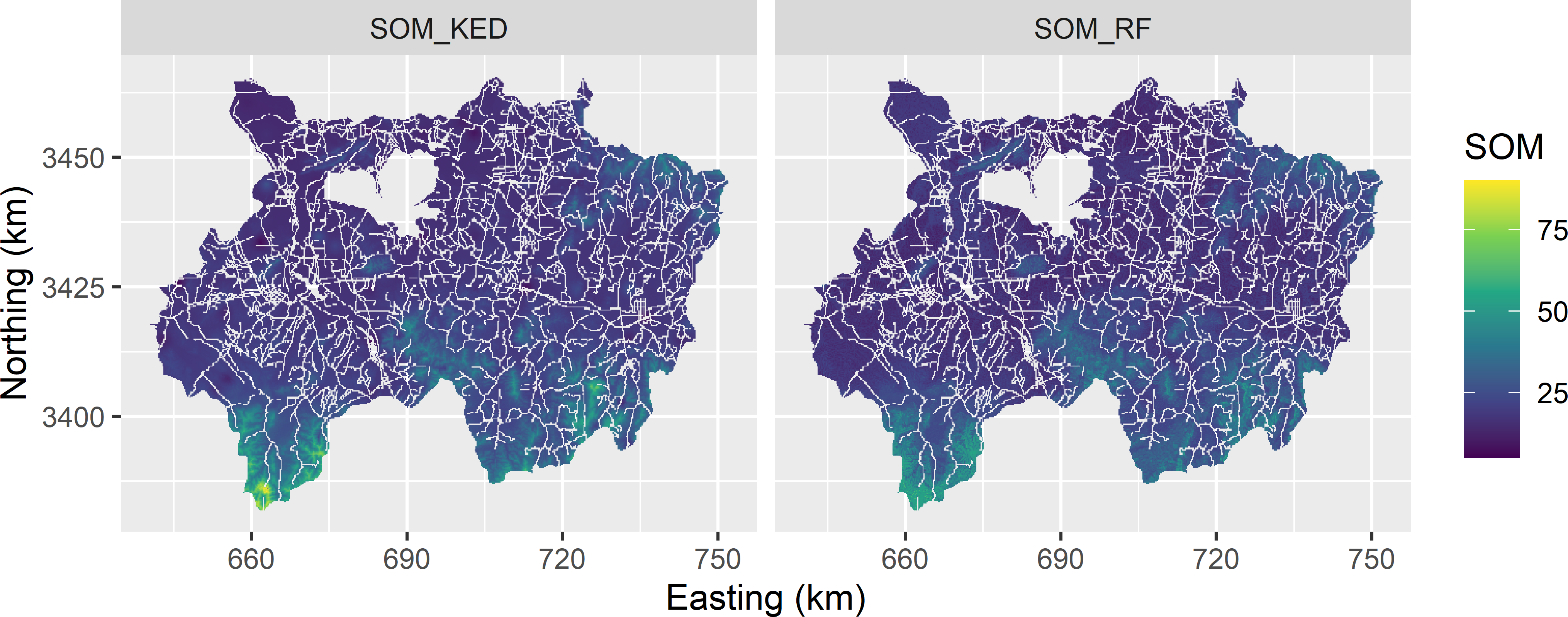
Figure 25.1: Map of the SOM concentration (g kg-1) in the topsoil of Xuancheng, obtained by kriging with an external drift (KED) and random forest (RF).
The two maps are evaluated by statistical validation with a stratified simple random sample of 62 units (points). The strata are the eight units of a geological map (Figure 25.2).
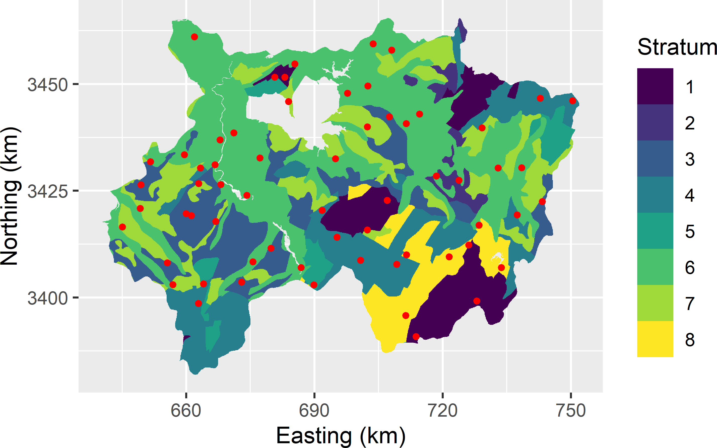
Figure 25.2: Stratified simple random sample for validation of the two maps of the SOM concentration in Xuancheng.
25.2.1 Estimation of the population mean error and mean squared error
To estimate the population MSE of the two maps, first the squared prediction errors are computed. The name of the measured study variable at the validation sample in data.frame sample_test is SOM_A_hori. Four new variables are added to sample_test using function mutate, by computing the prediction errors for KED and RF and squaring these errors.
sample_test <- read.csv(file = "results/STSI_Xuancheng_SOMpred.csv")
sample_test <- sample_test %>%
    mutate(
      eKED = SOM_A_hori - SOM_KED,
      eRF = SOM_A_hori - SOM_RF,
      e2KED = (SOM_A_hori - SOM_KED)^2,
      e2RF = (SOM_A_hori - SOM_RF)^2)
These four new variables now are our study variables of which we would like to estimate the population means. The population means can be estimated as explained in Chapter 4. First, the stratum sizes and stratum weights are computed, i.e., the number and relative number of raster cells per stratum (Figure 25.2).
rmap <- rast(x = system.file("extdata/Geo_Xuancheng.tif", package = "sswr"))
strata_Xuancheng <- as.data.frame(rmap, xy = TRUE, na.rm = TRUE) %>%
  rename(stratum = Geo_Xuancheng) %>%
  filter(stratum != 99) %>%
  group_by(stratum) %>%
  summarise(N_h = n()) %>%
  mutate(w_h = N_h / sum(N_h))
Next, the stratum means of the prediction errors, obtained with KED and RF, are estimated by the sample means, and the population mean of the errors are estimated by the weighted mean of the estimated stratum means.
me <- sample_test %>%
    group_by(stratum) %>%
    summarise(
      meKED_h = mean(eKED),
      meRF_h = mean(eRF)) %>%
    left_join(strata_Xuancheng, by = "stratum") %>%
    summarise(
      meKED = sum(w_h * meKED_h),
      meRF = sum(w_h * meRF_h))
This is repeated for the squared prediction errors.
mse <- sample_test %>%
    group_by(stratum) %>%
    summarise(
      mseKED_h = mean(e2KED),
      mseRF_h = mean(e2RF)) %>%
    left_join(strata_Xuancheng, by = "stratum") %>%
    summarise(
      mseKED = sum(w_h * mseKED_h),
      mseRF = sum(w_h * mseRF_h))
The estimated MSE of the KED map equals 89.3 (g kg-1)2, that of the RF map 93.8 (g kg-1)2.
25.2.2 Estimation of the standard error of the estimator of the population mean error and mean squared error
We are uncertain about both population MSEs, as we measured the squared errors at 62 sampling points only. So, we would like to know how uncertain we are. This uncertainty is quantified by the standard error of the estimator of the population MSE. A problem is that in the second stratum we have only one sampling point. So, for this stratum we cannot compute the variance of the squared errors. To compute the variance, we need at least two sampling points.
# A tibble: 8 x 2
  stratum     n
    <int> <int>
1       1     5
2       2     1
3       3     8
4       4    10
5       5     2
6       6    23
7       7     9
8       8     4
A solution is to merge stratum 2 with stratum 1, which is a similar geological map unit (we know this from the domain expert). This is referred to as collapsing the strata. An identifier for the collapsed strata is added to n_strata. This table is subsequently used to add the collapsed stratum identifiers to sample_test and strata_Xuancheng.
n_strata <- n_strata %>%
    mutate(stratum_clp = c(1, 1:7))
sample_test <- sample_test %>%
    left_join(n_strata, by = "stratum")
strata_Xuancheng <- strata_Xuancheng %>%
    left_join(n_strata, by = "stratum")
The collapsed strata can be used to estimate the standard errors of the estimators of the population MSEs. As a first step, the weights and the sample sizes of the collapsed strata are computed.
strata_clp_Xuancheng <- strata_Xuancheng %>%
    group_by(stratum_clp) %>%
    summarise(N_hc = sum(N_h)) %>%
    mutate(w_hc = N_hc / sum(N_hc)) %>%
    left_join(
      sample_test %>%
        group_by(stratum_clp) %>%
        summarise(n_hc = n()),
      by = "stratum_clp")
The sampling variance of the estimator of the mean of the (squared) prediction error can be estimated by Equation (4.4). The estimated ME and MSE and their estimated standard errors are shown in Table 25.1.
se <- sample_test %>%
    group_by(stratum_clp) %>%
    summarise(
      s2e_KED_hc = var(eKED),
      s2e2_KED_hc = var(e2KED),
      s2e_RF_hc = var(eRF),
      s2e2_RF_hc = var(e2RF)) %>%
    left_join(strata_clp_Xuancheng, by = "stratum_clp") %>%
    summarise(
      se_me_KED = sqrt(sum(w_hc^2 * s2e_KED_hc / n_hc)),
      se_mse_KED = sqrt(sum(w_hc^2 * s2e2_KED_hc / n_hc)),
      se_me_RF = sqrt(sum(w_hc^2 * s2e_RF_hc / n_hc)),
se_mse_RF = sqrt(sum(w_hc^2 * s2e2_RF_hc / n_hc)))| KED | seKED | RF | seRF | |
|---|---|---|---|---|
| ME | 0.83 | 1.2 | 0.4 | 1.29 |
| MSE | 89.30 | 25.5 | 93.8 | 25.80 |
25.2.3 Estimation of model efficiency coefficient
To estimate the MEC, we must first estimate the population variance of the study variable from the stratified simple random sample (the denominator in Equation (25.7)). First, the sizes and the sample sizes of the collapsed strata must be added to sample_test. Then the population variance is estimated with function s2 of package surveyplanning (Subsection 4.1.2).
library(surveyplanning)
s2z <- sample_test %>%
  left_join(strata_clp_Xuancheng, by = "stratum_clp") %>%
  summarise(s2z = s2(SOM_A_hori, w = N_hc / n_hc)) %>%
  flatten_dbl
Now the MECs for KED and RF can be estimated.
The estimated MEC for KED equals 0.016 and for RF -0.034, showing that the two models used in mapping are no better than the estimated mean SOM concentration used as a predictor. This is quite a disappointing result.
25.2.4 Statistical testing of hypothesis about population ME and MSE
The hypothesis that the population ME equals 0 can be tested by a one-sample t-test. The alternative hypothesis is that ME is unequal to 0 (two-sided alternative). The number of degrees of freedom of the t distribution is approximated by the total sample size minus the number of strata (Section 4.2). Note that we have a two-sided alternative hypothesis, so we must compute a two-sided p-value.
t_KED <- me$meKED / se$se_me_KED
df <- nrow(sample_test) - length(unique(sample_test$stratum_clp))
p_KED <- 2 * pt(t_KED, df = df, lower.tail = t_KED < 0)
The outcomes of the test statistics are 0.690 and 0.309 for KED and RF, respectively, with p-values 0.493 and 0.759. So, we clearly have not enough evidence for systematic errors, neither with KED nor with RF mapping.
Now we test whether the two population MSEs differ significantly. This can be done by a paired t-test. The first step in a paired t-test is to compute pairwise differences of squared prediction errors, and then we can proceed as in a one-sample t-test.
m_de2 <- sample_test %>%
  mutate(de2 = e2KED - e2RF) %>%
  group_by(stratum) %>%
  summarise(m_de2_h = mean(de2)) %>%
  left_join(strata_Xuancheng, by = "stratum") %>%
  summarise(m_de2 = sum(w_h * m_de2_h)) %>%
  flatten_dbl

se_m_de2 <- sample_test %>%
  mutate(de2 = e2KED - e2RF) %>%
  group_by(stratum_clp) %>%
  summarise(s2_de2_hc = var(de2)) %>%
  left_join(strata_clp_Xuancheng, by = "stratum_clp") %>%
  summarise(se_m_de2 = sqrt(sum(w_hc^2 * s2_de2_hc / n_hc))) %>%
  flatten_dbl

t <- m_de2 / se_m_de2
p <- 2 * pt(t, df = df, lower.tail = t < 0)
The outcome of the test statistic is -0.438, with a p-value of 0.663, so we clearly do not have enough evidence that the population MSEs obtained with the two mapping methods are different.