Chapter 24 Sampling for estimating the semivariogram
For model-based sampling as described in Chapters 22 and 23, we must specify the (residual) semivariogram. In case we do not have a reasonable prior estimate of the semivariogram, we may decide to first collect data with the specific aim of estimating the semivariogram. This semivariogram is subsequently used to design a model-based sample for mapping. This chapter is about how to design a reconnaissance sample survey for estimating the semivariogram.
The first question is how many observations we need for this. Webster and Oliver (1992) gave as a rule of thumb that 150 to 225 points are needed to obtain a reliable semivariogram when estimated by the method-of-moments (MoM). Lark (2000) showed that with maximum likelihood (ML) estimation two-thirds to only half of the observations are needed to achieve equal precision of the estimated semivariogram parameters.
Once we have decided on the sample size, we must select the locations of the sampling units. Two random sampling designs for semivariogram estimation are described, nested sampling (Section 24.1) and independent sampling of pairs of points (Section 24.2). Section 24.3 is devoted to model-based optimisation of the sampling pattern for semivariogram estimation. Section 24.4 is about how to design a single sample that can be used both for estimation of the semivariogram and prediction (mapping). In a final section, a practical solution is described for the problem of how to design a sample for semivariogram estimation and prediction.
24.1 Nested sampling
Nested sampling can be used to estimate the semivariance at a limited number of separation distances, see Oliver and Webster (1986) and Webster et al. (2006). First, we must decide on these separation distances. We need point-pairs at various separation distances, especially for small separation distances, so that we get reliable estimates of this part of the semivariogram which has a strong effect on the kriging weights. Usually, separation distances are chosen in a geometric progression, for instance 2, 8, 32, 128, and 512 m. The multiplier, which is four in this example, should not be too small; as a rule of thumb, use three or larger.
There are two versions of nested sampling. In the first stage of the first version, several main stations are selected in a way that they cover the study area well, for instance by spatial coverage sampling. In the second stage, each of the main stations is used as a starting point to select one point at a distance equal to the largest chosen separation distance (512 m in the example) in a random direction from the main station. This doubles the sample size. In the third stage, all points selected in the previous stages (main stations of stage 1 plus the points of stage 2) are used as starting points to select one point at a distance equal to the second largest separation distance (128 m), and so on. All points selected in the various stages are included in the nested sample. The code chunk below shows the function for random selection of one point at distance \(h\) from a starting point. Note the while loop which continues until a point is found that is inside the area. This is checked with function over of package sp.
SelectPoint <- function(start, h, area) {
  dxy <- numeric(length = 2)
  inArea <- NA
  while (is.na(inArea)) {
    angle <- runif(n = 1, min = 0, max = 2 * pi)
    dxy[1] <- h * sin(angle); dxy[2] <- h * cos(angle)
    xypnt <- start + dxy
    coordinates(xypnt) <- ~ s1 + s2
    inArea <- as.numeric(over(x = xypnt, y = area))[1]
  }
  xypoint <- as.data.frame(xypnt)
  xypoint
}
The first stage of the second version is equal to that of the first version. However, in the second stage each of the main stations serves as a starting point for randomly selecting a pair of points with a separation distance equal to the largest chosen separation distance. The main station is halfway the selected pair of points. In the third stage, each of the substations is used to select in the same way a pair of points separated by the second largest chosen distance, and so on. Only the points selected in the final stage are used as sampling points. The R code below shows the function for random selection of two points separated by \(h\) distance units with a starting point halfway the pair of points. The while loop continues until both points of a pair are inside the area.
SelectPair <- function(start, h, area) {
  dxy <- numeric(length = 2)
  xypoints <- NULL
  inArea1 <- inArea2 <- NA
  while (is.na(inArea1) | is.na(inArea2)) {
    angle <- runif(n = 1, min = 0, max = 2 * pi)
    dxy[1] <- h * sin(angle) / 2; dxy[2] <- h * cos(angle) / 2
    xypnt1 <- start + dxy
    coordinates(xypnt1) <- ~ s1 + s2
    inArea1 <- as.numeric(over(x = xypnt1, y = area))[1]
    dxy[1] <- -dxy[1]; dxy[2] <- -dxy[2]
    xypnt2 <- start + dxy
    coordinates(xypnt2) <- ~ s1 + s2
    inArea2 <- as.numeric(over(x = xypnt2, y = area))[1]
  }
  xypoints <- rbind(as.data.frame(xypnt1), as.data.frame(xypnt2))
  xypoints
}
The R code below shows the selection of a nested sample from Hunter Valley using both versions. Only one main station is selected. In total 16 points are selected in four stages. The separation distances are 2,000, 1,000, 500, and 250 m. Sixteen points is not enough for estimating the semivariogram and a multiplier of two is rather small, but this example is for illustrative purposes only.
Note that the separation distances are in descending order. The largest separation distance should not be chosen too large, because then, when the main station is somewhere in the middle of the study area, it may happen that using the first version, no pair can be found with that separation distance. A similar problem may occur with the second version when in subsequent stages a station is selected near the border of the study area. A copy of grdHunterValley is made because both the original data frame is needed, as well as a gridded version of this data frame.
library(sp)
grid <- grdHunterValley
gridded(grdHunterValley) <- ~ s1 + s2
lags <- c(2000, 1000, 500, 250)
The next code chunk is an implementation of the first version of nested sampling.
set.seed(614)
unit <- sample(nrow(grid), 1)
mainstation <- grid[unit, c("s1", "s2")]
newpnt <- SelectPoint(start = mainstation, h = lags[1], area = grdHunterValley)
mysample_nested <- rbind(mainstation, newpnt)
for (j in 2:length(lags)) {
  newpnts <- NULL
  for (i in seq_len(nrow(mysample_nested))) {
    pnts <- SelectPoint(
      start = mysample_nested[i, ], h = lags[j], area = grdHunterValley)
    newpnts <- rbind(newpnts, pnts)
  }
  mysample_nested <- rbind(mysample_nested, newpnts)
}
The R code for the second version is presented in the next code chunk.
unit <- sample(nrow(grid), 1)
mainstation <- grid[unit, c("s1", "s2")]
pnt <- SelectPoint(start = mainstation, h = lags[1], area = grdHunterValley)
stations <- rbind(mainstation, pnt)
allstations <-  rbind(mainstation, pnt)
for (j in 2:length(lags)) {
  newstations <- NULL
  for (i in seq_len(nrow(stations))) {
    pnts <- SelectPair(
      start = stations[i, ], h = lags[j], area = grdHunterValley)
    newstations <- rbind(newstations, pnts)
    allstations <- rbind(allstations, pnts)
  }
  stations <- newstations
}
mysample_nested_2 <- as_tibble(stations)
Figure 24.1 shows the two selected nested samples. For the sample selected with the second version, also the stations that served as starting points for the selection of the point-pairs are plotted.
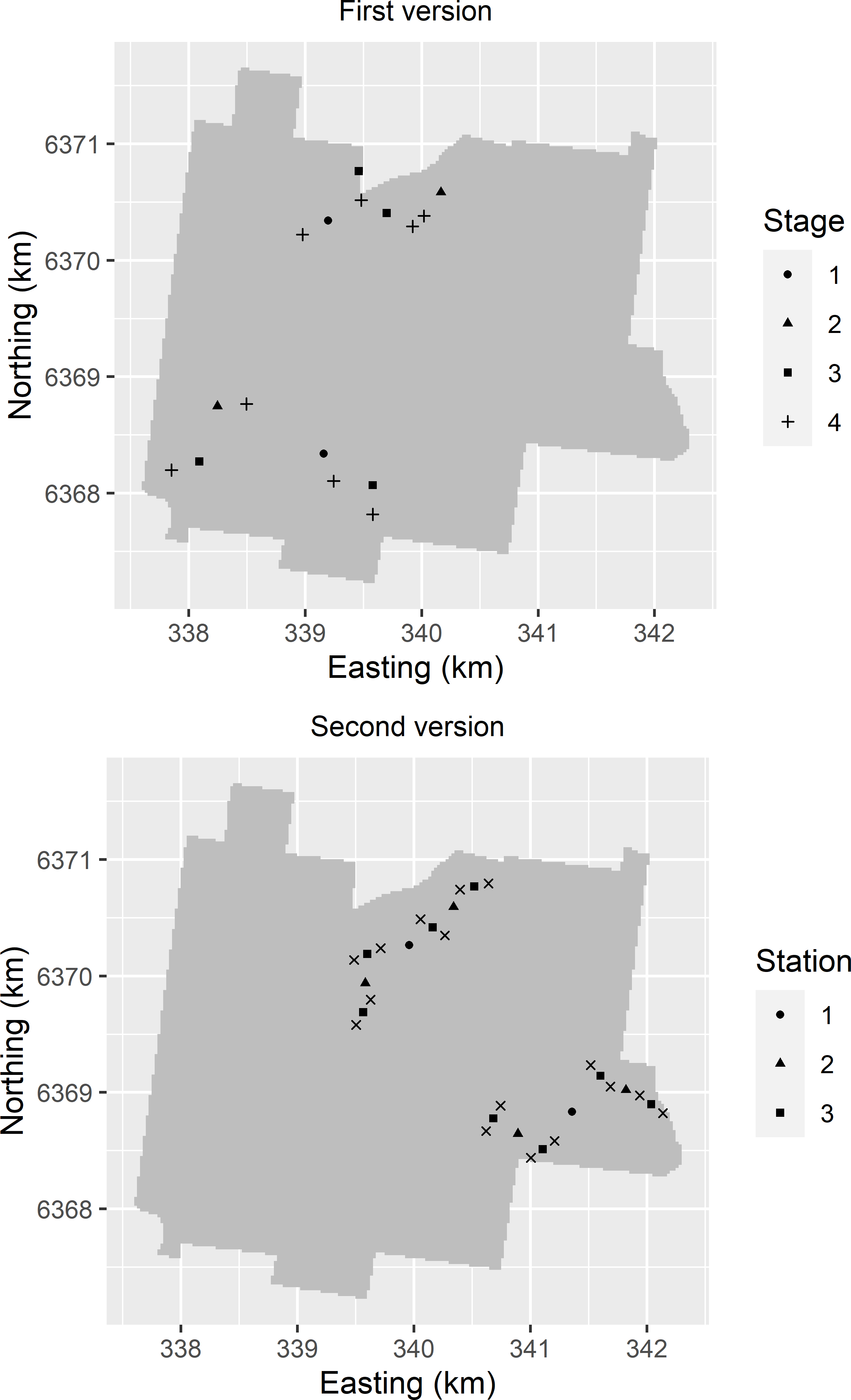
Figure 24.1: Balanced nested samples from Hunter Valley, selected with the two versions of nested sampling. In the subfigure of the second version the selected sampling points (symbol x) are plotted together with the selected stations (halfway the two points of a pair).
The samples of Figure 24.1 are examples of balanced nested samples. The number of point-pairs separated by a given distance doubles with every stage. As a consequence, the estimated semivariances for the smallest separation distance are much more precise than for the largest distance. We are most uncertain about the estimated semivariances for the largest separation distances. If in the first stage only one point-pair separated by the largest distance is selected, then we have only one degree of freedom for estimating the variance component associated with this stage. It is more efficient to select more than one main station, say about ten, and to select fewer points in the final stages. For instance, with the second version we may decide to select a point-pair at only half the number of stations selected in the one-but-last stage. The nested sample then becomes unbalanced.
The model for nested sampling with four stages is a hierarchical analysis of variance (ANOVA) model with random effects:
\[\begin{equation} Z_{ijkl}=\mu+A_i+B_{ij}+C_{ijk}+\epsilon_{ijkl} \;, \tag{24.1} \end{equation}\]
with \(\mu\) the mean, \(A_i\) the effect of the \(i\)th first stage station, \(B_{ij}\) the effect of the \(j\)th second stage station within the \(i\)th first stage station, and so on. \(A_i\), \(B_{ij}\), \(C_{ijk}\), and \(\epsilon_{ijkl}\) are random quantities (random effects) all with zero mean and variances \(\sigma^2_1\), \(\sigma^2_2\), \(\sigma^2_3\), and \(\sigma^2_4\), respectively.
For balanced designs, the variance components can be estimated by the MoM from a hierarchical ANOVA. The first step is to assign factors to the sampling points that indicate the grouping of the sampling points in the various stages. The number of factors needed is the number of stages minus 1. All factors have two levels. Figures 24.2 and 24.3 show the levels of the three factors. The levels of the first factor show the strongest spatial clustering, those of the second factor the one-but-strongest, and so on.
mysample_nested$factor1 <- rep(rep(1:2), times = 8)
mysample_nested$factor2 <- rep(rep(1:2, each = 2), times = 4)
mysample_nested$factor3 <- rep(rep(1:2, each = 4), times = 2)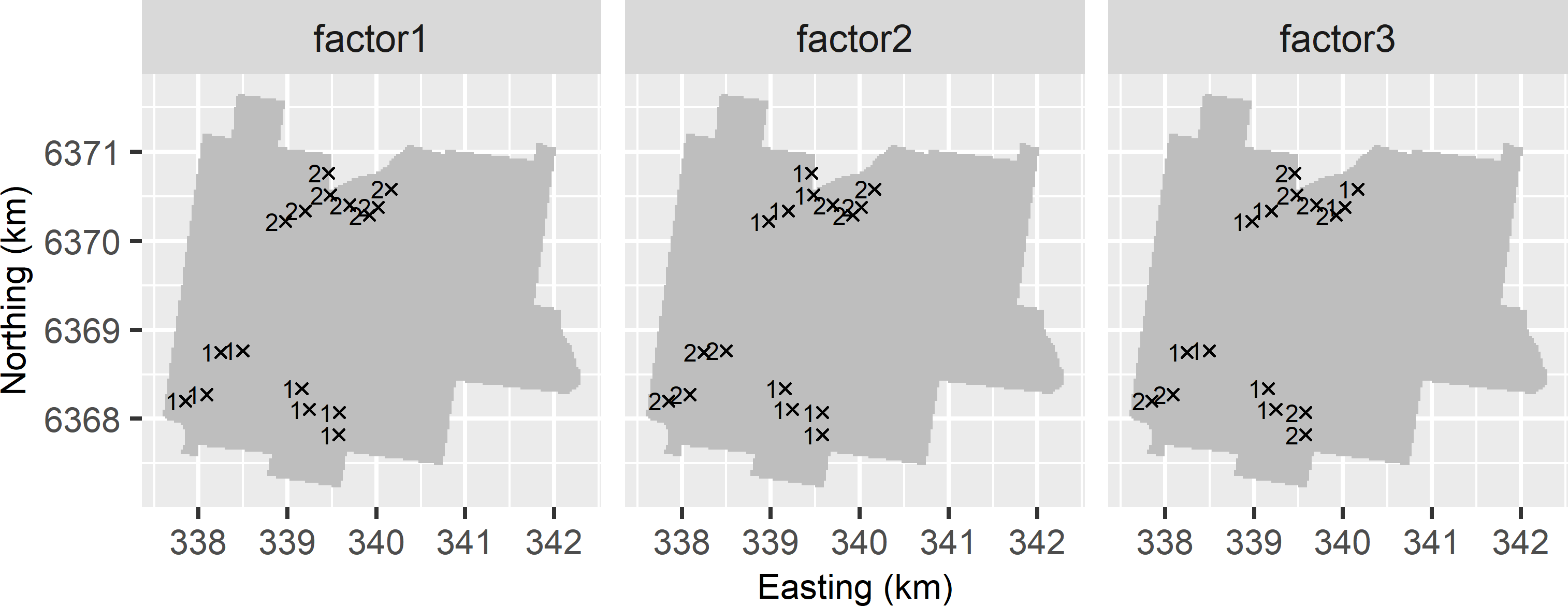
Figure 24.2: The levels of the three factors assigned to the sampling points of the balanced nested sample selected with the first version.
The R code below shows the construction of the three factors for the second version of nested sampling.
mysample_nested_2$factor1 <- rep(1:2, each = 8)
mysample_nested_2$factor2 <- rep(rep(1:2, each = 4), times = 2)
mysample_nested_2$factor3 <- rep(rep(1:2, each = 2), times = 4)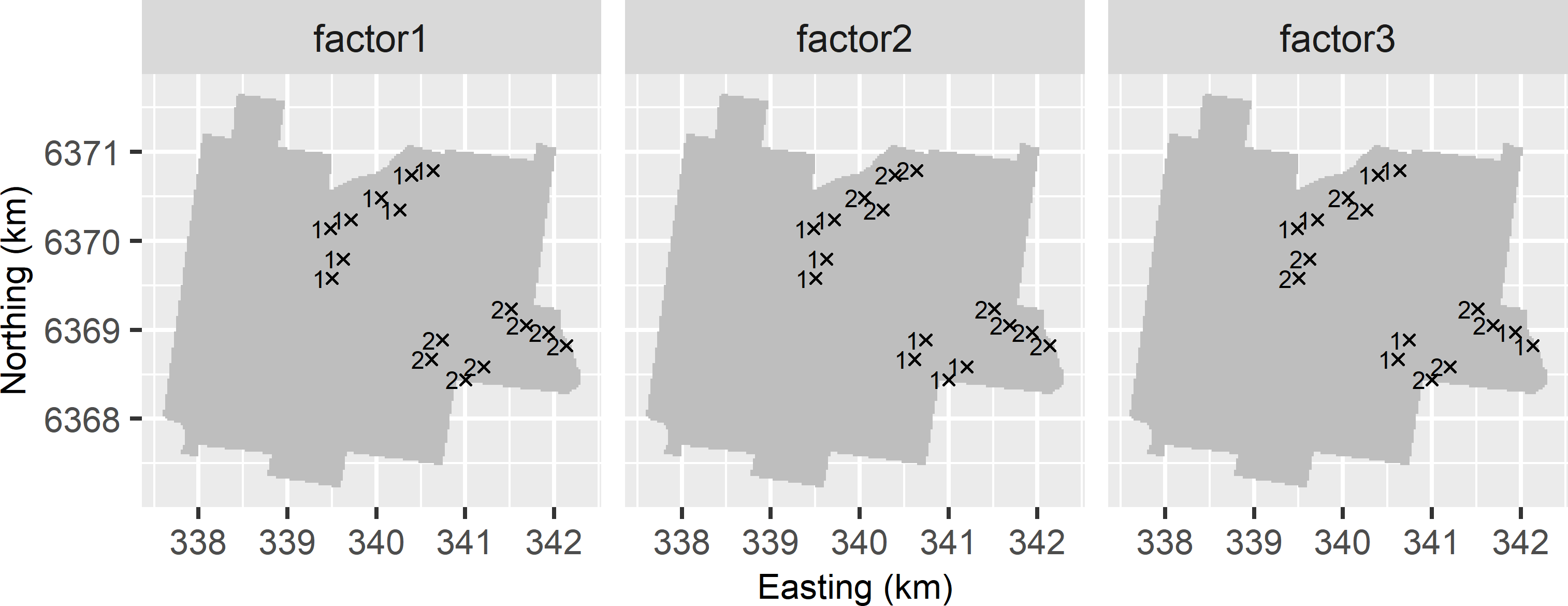
Figure 24.3: The levels of the three factors assigned to the sampling points of the balanced nested sample selected with the second version.
For unbalanced nested designs, the variance components can be estimated by restricted maximum likelihood (REML) (Webster et al. 2006). REML estimation is also recommended if in Equation (24.1) instead of a constant mean \(\mu\) the mean is a linear combination of one or more covariates (fixed effects). The semivariances at the chosen separation distances are obtained by cumulating the estimated variance components.
The R code below shows how the variance components and the semivariances can be estimated with function lme of the package nlme (Pinheiro et al. 2021), once the data are collected and added to the data frame. This function fits linear mixed-effects models and allows for nested random effects. It can be used both for balanced and unbalanced nested samples, and for a constant mean or a mean that is a linear combination of covariates. Argument fixed is a formula describing the fixed effects with the response variable on the left-hand side of the ~ operator and the covariates for the mean on the right-hand side. If a constant mean is assumed, as in our example, this is indicated by the 1 on the right-hand side of the ~ operator. Argument random is a one-sided formula (no response variable is on the left-hand side of the ~ operator). On the right-hand side of the \(|\) separator, the nested structure of the data is specified using the factors of Figure 24.2. The 1 on the left-hand side of the \(|\) separator means that we assume that all regression coefficients associated with the covariates are fixed (non-random) quantities.
library(nlme)
lmodel <- lme(
  fixed = z ~ 1, data = mysample_nested,
  random = ~ 1 | factor1 / factor2 / factor3)
res <- as.matrix(VarCorr(lmodel))
sigmas <- as.numeric(res[c(2, 4, 6, 7), 1])
sigma <- rev(sigmas)
semivar <- cumsum(sigmas)
Random sampling of the points is not strictly needed, because a model-based approach is followed here. The model of Equation (24.1) is a superpopulation model, i.e., we assume that the population is generated by this model (see Chapter 26). Papritz et al. (2011), for instance, selected the points (using the second version) non-randomly to improve the control of the nested subareas and the average separation distances.
Lark (2011) describes a method for optimisation of a nested design, given the total number of points and the chosen separation distances.
Exercises
- Write an R script to select with the first version a balanced nested sample from Hunter Valley. Use as separation distances 1,000, 500, 200, 100, and 50 m.
- Add the factors that are needed for estimating the variance components to the data frame with the selected sampling points.
- Overlay the sampling points with the
SpatialPixelsDataFrame, and estimate the semivariances for the attribute compound topographic index (cti).
24.2 Independent sampling of pairs of points
With the nested design, the estimated semivariances for the different separation distances are not independent. Independent estimated semivariances can be obtained by independent random selection of pairs of points (IPP sampling). Independence here means design-independence, see Section 26.2. Similar to a regression model, a semivariogram can be defined as a superpopulation model or as a population model. Only in the current section a semivariogram is defined at the population level. Such a semivariogram is referred to as a non-ergodic semivariogram or local semivariogram (Brus and de Gruijter 1994).
IPP sampling is straightforward for simple random sampling. For each separation distance a point-pair is selected by first selecting fully randomly one point from the study area. Then the second point is randomly selected from the circle with the first point at its centre and a radius equal to the chosen separation distance. If this second point is outside the study area, both points are discarded. This is repeated until we have the required point-pairs for this separation distance. The next code chunk is an implementation of this selection procedure.
SIpairs <- function(h, n, area) {
  topo <- as(getGridTopology(area), "data.frame")
  cell_size <- topo$cellsize[1]
  xy <- coordinates(area)
  dxy <- numeric(length = 2)
  xypnts1 <- xypnts2 <- NULL
  i <- 1
  while (i <= n) {
    unit1 <- sample(length(area), size = 1)
    xypnt1 <- xy[unit1, ]
    xypnt1[1] <- jitter(xypnt1[1], amount = cell_size / 2)
    xypnt1[2] <- jitter(xypnt1[2], amount = cell_size / 2)
    angle <- runif(n = 1, min = 0, max = 2 * pi)
    dxy[1] <- h * sin(angle); dxy[2] <- h * cos(angle)
    xypnt2 <- as.data.frame(t(xypnt1 + dxy))
    coordinates(xypnt2) <- ~ s1 + s2
    inArea <- as.numeric(over(x = xypnt2, y = area))[1]
    if (!is.na(inArea)) {
      xypnts1 <- rbind(xypnts1, xypnt1)
      xypnts2 <- rbind(xypnts2, as.data.frame(xypnt2))
      i <- i + 1
    }
    rm(xypnt1, xypnt2)
  }
  cbind(xypnts1, xypnts2)
}
IPP sampling is illustrated with the compound topographic index (cti, which is the same as topographic wetness index) data of Hunter Valley. Five separation distances are chosen, collected in numeric h, and for each distance \(n=100\) point-pairs are selected by simple random sampling.
library(sp)
h <- c(50, 100, 200, 500, 1000)
n <- 100
set.seed(123)
allpairs <- NULL
for (i in seq_len(length(h))) {
  pairs <- SIpairs(h = h[i], n = n, area = grdHunterValley)
  allpairs <- rbind(allpairs, pairs, make.row.names = FALSE)
}
The data.frame allpairs has four variables: the spatial coordinates of the first and of the second point of a pair. An overlay is made of the selected points with the SpatialPixelsDataFrame, and the cti values are extracted.
pnt1 <- allpairs[, c(1, 2)]
coordinates(pnt1) <- ~ s1 + s2
z1 <- over(x = pnt1, y = grdHunterValley)["cti"]
pnt2 <- allpairs[, c(3, 4)]
coordinates(pnt2) <- ~ s1 + s2
z2 <- over(x = pnt2, y = grdHunterValley)["cti"]
mysample <- data.frame(h = rep(h, each = n), z1, z2)
names(mysample)[c(2, 3)] <- c("z1", "z2")
The semivariances for the chosen separation distances are estimated as well as the variance of these estimated semivariances.
gammah <- vgammah <- numeric(length = length(h))
for (i in seq_len(length(h))) {
  units <- which(mysample$h == h[i])
  pairsh <- mysample[units, ]
  gammah[i] <- mean((pairsh$z1 - pairsh$z2)^2, na.rm = TRUE) / 2
  vgammah[i] <- var((pairsh$z1 - pairsh$z2)^2, na.rm = TRUE) / (n * 4)
}
A spherical model with nugget is fitted to the sample semivariogram, using function nls, with weights equal to the reciprocal of the estimated variances of the estimated semivariances.
sample_vg <- data.frame(h, gammah, vgammah)
SphNug <- function(h, range, psill, nugget) {
  h <- h / range
  nugget + psill * ifelse(h < 1, (1.5 * h - 0.5 * h^3), 1)
}
fit.var <- nls(gammah ~ SphNug(h, range, psill, nugget),
  data = sample_vg, start = list(psill = 4, range = 200, nugget = 1),
  weights = 1 / vgammah, algorithm = "port", lower = c(0, 0, 0))
print(pars <- signif(coef(fit.var), 3))
psill range nugget
3.29 188.00 1.21 Figure 24.4 shows the sample semivariogram and the fitted model.
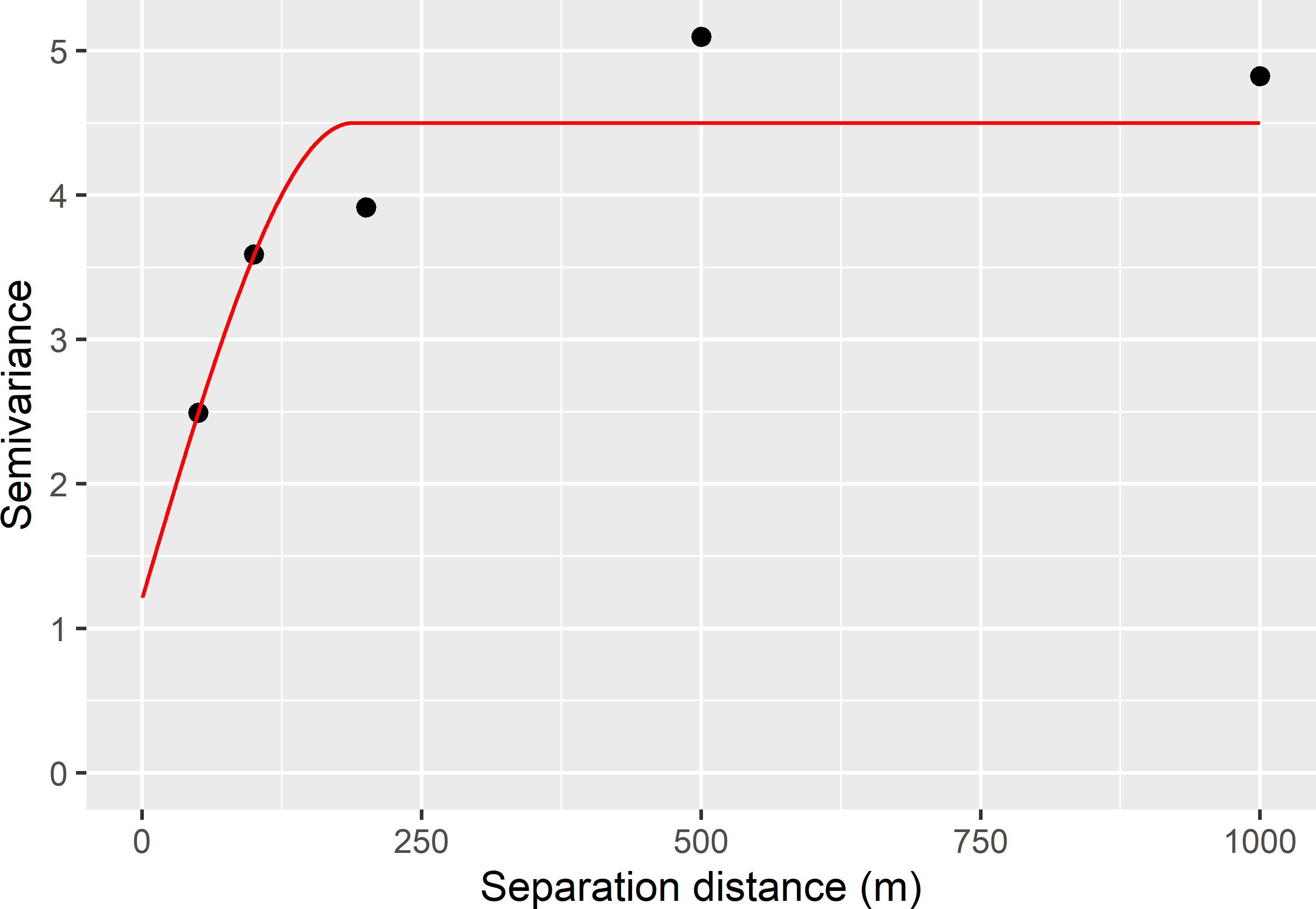
Figure 24.4: Sample semivariogram, obtained by independent sampling of pairs of points, and fitted spherical model of compount topographic index in Hunter Valley.
The covariances of the estimated semivariances at different separation distances are zero, as the point-pairs are selected independently. This keeps estimation of the variances and covariances of the estimated semivariogram parameters simple. In the next code chunk, this is done by bootstrapping.
In bootstrapping, for each separation distance a simple random sample with replacement of point-pairs is selected from the original sample of point-pairs. A point-pair can be selected more than once. The sample size (number of draws) is equal to the total number of point-pairs per separation distance in the original sample.
Every run of the bootstrap results in as many bootstrap samples as there are separation distances. The bootstrap samples are used to fit a semivariogram model. The whole procedure is repeated 500 times, resulting in 500 vectors with model parameters. These vectors can be used to estimate the variances and covariances of the estimators of the three semivariogram parameters.
allpars <- NULL
R <- 500
for (j in 1:R) {
  gammah <- vgammah <- numeric(length = length(h))
  for (i in seq_len(length(h))) {
    units <- which(mysample$h == h[i])
    mysam_btsp <- mysample[units, ] %>%
      slice_sample(n = n, replace = TRUE)
    gammah[i] <- mean((mysam_btsp$z1 - mysam_btsp$z2)^2, na.rm = TRUE) / 2
    vgammah[i] <- var((mysam_btsp$z1 - mysam_btsp$z2)^2, na.rm = TRUE) / (n * 4)
  }
  sample_vg <- data.frame(h, gammah, vgammah)
  tryCatch({
    fittedvariogram <- nls(gammah ~ SphNug(h, range, psill, nugget),
    data = sample_vg, start = list(psill = 4, range = 200, nugget = 1),
    weights = 1 / vgammah, algorithm = "port", lower = c(0, 0, 0))
  pars <- coef(fittedvariogram)
  allpars <- rbind(allpars, pars)}, error = function(e) {})
}
#compute variance-covariance matrix
signif(var(allpars), 3)
psill range nugget
psill 1.160 -44.6 -0.803
range -44.600 66700.0 172.000
nugget -0.803 172.0 1.070Note the large variance for the range parameter (the standard deviation is 258 m) as well as the negative covariance of the nugget and the partial sill parameter (the Pearson correlation coefficient is -0.72). Histograms of the three estimated semivariogram parameters are shown in Figure 24.5.
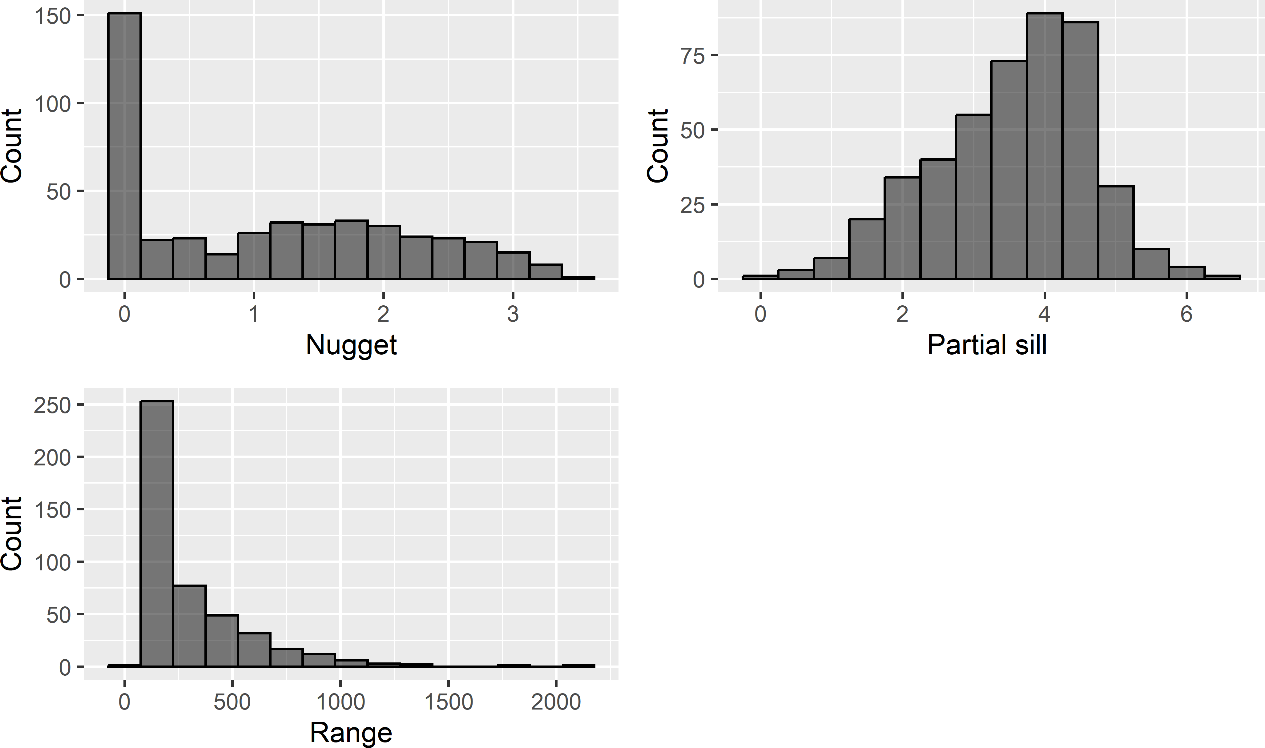
Figure 24.5: Frequency distributions of estimated parameters of a spherical semivariogram of compound topographic index in Hunter Valley.
Exercises
- Write an R script to select simple random samples of pairs of points for estimating the semivariogram of cti in Hunter Valley. Use as separation distances 25, 50, 100, 200, and 400 m. Note that these separation distances are smaller than those used above. Select 100 pairs per separation distance.
- Compute the sample semivariogram, and estimate a spherical model with nugget using function
nls. - Compare the estimated semivariogram parameters with the estimates obtained with the larger separation distances.
- Estimate the variance-covariance matrix of the estimated semivariogram parameters by bootstrapping.
- Compare the variances of the estimated semivariogram parameters with the variances obtained with the larger separation distances. Which variance is changed most?
- Compute the sample semivariogram, and estimate a spherical model with nugget using function
24.3 Optimisation of sampling pattern for semivariogram estimation
There is rich literature on model-based optimisation of the sampling locations for semivariogram estimation. Several design criteria (minimisation criteria) have been proposed for optimising the sampling pattern. Various authors have proposed a measure of the uncertainty about the semivariogram parameters as a minimisation criterion. These criteria are described and illustrated in the next subsection. The kriging variance is sensitive to errors in the estimated semivariogram. Therefore, Lark (2002) proposed to use a measure of the uncertainty about the kriging variance as a minimisation criterion (Subsection 24.3.2).
24.3.1 Uncertainty about semivariogram parameters
W. G. Müller and Zimmerman (1999) as well as Bogaert and Russo (1999) proposed the determinant of the variance-covariance matrix of semivariogram parameters, estimated by generalised least squares to fit the MoM sample semivariogram. For instance, if we have two semivariogram parameters, \(\theta_1\) and \(\theta_2\), the determinant of the 2 \(\times\) 2 variance-covariance matrix equals the sum of the variances of the two estimated parameters minus two times the covariance of the two estimated parameters. If the two estimated parameters are positively correlated, the determinant of the matrix is smaller than if they are uncorrelated, and the covariance term is zero. The determinant is a measure of our joint uncertainty about the semivariogram parameters.
Zhu and Stein (2005) proposed as a minimisation criterion the log of the determinant of the inverse Fisher information matrix in ML estimation of the semivariogram, hereafter shortly denoted by logdet. The Fisher information about a semivariogram parameter is a function of the likelihood of the semivariogram parameter; the likelihood of a semivariogram parameter is the probability of the data as a function of the semivariogram parameter. The log of this likelihood can be plotted against values of the parameter. The flatter the log-likelihood surface, the less information is in the data about the parameter. The flatness of the surface can be measured by the first derivative of the log-likelihood to the semivariogram parameter. Strong negative or positive derivative values indicate a steep surface. The Fisher information for a model parameter is defined as the expectation of the square of the first derivative of the log-likelihood to that semivariogram parameter, see Ly et al. (2017) for a nice tutorial on this subject. The more information we have about a semivariogram, the less uncertain we are about that parameter. This explains why the inverse of the Fisher information can be used as a measure of uncertainty. The inverse Fisher information matrix contains the variances and covariances of the estimated semivariogram parameters.
The code chunks hereafter show how logdet can be computed. It makes use of the result of Kitanidis (1987) who showed that each element of the Fisher information matrix \(\mathbf{I}(\theta)\) can be obtained with (see also Lark (2002))
\[\begin{equation} [\mathbf{I}(\theta)]_{ij}=\frac{1}{2}\mathrm{Tr}\left[\mathbf{A}^{-1}\frac{\partial\mathbf{A}}{\partial\theta_i}\mathbf{A}^{-1}\frac{\partial\mathbf{A}}{\partial\theta_j}\right]\;, \tag{24.2} \end{equation}\]
with \(\mathbf{A}\) the correlation matrix of the sampling points, \(\frac{\partial\mathbf{A}}{\partial\theta_i}\) the partial derivative of the correlation matrix to the \(i\)th semivariogram parameter, and Tr[\(\cdot\)] the trace of a matrix.
As an illustration, I selected a simple random sample of 50 points from Hunter Valley. A matrix with distances between the points of a sample is computed. Preliminary values for the semivariogram parameters \(\xi\) (ratio of spatial dependence) and \(\phi\) (distance parameter) are obtained by visual inspection of the sample semivariogram, and the gstat (E. J. Pebesma 2004) function variogramLine is used to compute the correlation matrix.
library(sp)
library(gstat)
set.seed(314)
mysample0 <- grdHunterValley %>%
  slice_sample(n = 50)
coordinates(mysample0) <- ~ s1 + s2
D <- spDists(mysample0)
xi <- 0.8; phi <- 200
thetas <- c(xi, phi)
vgmodel <- vgm(model = "Exp", psill = thetas[1],
  range = thetas[2], nugget = 1 - thetas[1])
A <- variogramLine(vgmodel, dist_vector = D, covariance = TRUE)
In the next step, the semivariogram parameters are slightly changed one-by-one. The changes, referred to as perturbations, are a small fraction of the preliminary semivariogram parameter values. The perturbed semivariogram parameters are used to compute the perturbed correlation matrices (pA) and the partial derivatives of the correlation matrix (dA) for each perturbation.
perturbation <- 0.01
pA <- dA <- list()
for (i in seq_len(length(thetas))) {
  thetas_pert <- thetas
  thetas_pert[i] <- (1 + perturbation) * thetas[i]
  vgmodel_pert <- vgm(model = "Exp", psill = thetas_pert[1],
    range = thetas_pert[2], nugget = 1 - thetas_pert[1])
  pA[[i]] <- variogramLine(vgmodel_pert, dist_vector = D, covariance = TRUE)
  dA[[i]] <- (pA[[i]] - A) / (thetas[i] * perturbation)
}
Finally, the Fisher information matrix is computed using Equation (24.2). We do not need to compute the inverse of the Fisher information matrix, because the determinant of the inverse of a matrix is equal to the inverse of the determinant of the (not inverted) matrix. The determinant is computed with function determinant.
I <- matrix(0, length(thetas), length(thetas))
for (i in seq_len(length(thetas))) {
  m_i <- solve(A, dA[[i]])
  for (j in i:length(thetas)) {
    m_j <- solve(A, dA[[j]])
    I[i, j] <- I[j, i] <- 0.5 * sum(diag(m_i %*% m_j))
  }
}
logdet0 <- -determinant(I, logarithm = TRUE)$modulus
The joint uncertainty about the semivariogram parameters, as quantified by the log of the determinant of the inverse of the information matrix, equals 8.198. Hereafter, we will see how much this joint uncertainty can be reduced by optimising the spatial pattern of the sample used for semivariogram estimation, compared to the simple random sample used in the above calculation. Note that a preliminary semivariogram is needed to compute an optimised sampling pattern for semivariogram estimation.
Function optimUSER of package spsann can be used to search for the sampling locations with the minimum value of logdet. This function has been used before in Section 23.2. Package spsann cannot deal with the 22,124 candidate grid nodes of Hunter Valley; these are too many. I therefore selected a subgrid of 50 m \(\times\) 50 m.
The size of the sample for estimation of the semivariogram is passed to function optimUSER with argument points. The objective function to be minimised is passed to function optimUSER with argument fun. The objective function logdet is defined in package sswr. Argument model specifies the model type, using the characters for model types of package gstat. Argument thetas specifies the preliminary semivariogram parameter values. Argument perturbation specifies how much the semivariogram parameters are changed to compute the perturbed correlation matrices (pA) and the partial derivatives of the correlation matrix (dA).
gridded(grdHunterValley) <- ~ s1 + s2
candi <- spsample(grdHunterValley, type = "regular",
                  cellsize = c(50, 50), offset = c(0.5, 0.5))
candi <- as.data.frame(candi)
names(candi) <- c("x", "y")
schedule <- scheduleSPSANN(
  initial.acceptance = c(0.8, 0.95),
  initial.temperature = 0.15, temperature.decrease = 0.9,
  chains = 300, chain.length = 10, stopping = 10,
  x.min = 0, y.min = 0, cellsize = 50)
set.seed(314)
res <- optimUSER(
  points = 50, candi = candi,
  fun = logdet,
  model = "Exp", thetas = thetas, perturbation = 0.01,
  schedule = schedule, track = TRUE)
Figure 24.6 shows the optimised sampling pattern of 50 points. The logdet of the optimised sample equals 3.548, which is 43% of the value of the simple random sample used above to illustrate the computations. The optimised sample consists of two clusters. There are quite a few point-pairs with nearly coinciding points.
24.3.2 Uncertainty about the kriging variance
Lark (2002) proposed as a minimisation criterion the estimation variance of the kriging variance (VKV) due to uncertainty in the ML estimates of the semivariogram parameters. This variance is approximated by a first order Taylor series, requiring the partial derivatives of the kriging variance with respect to the semivariogram parameters:
\[\begin{equation} VKV(\mathbf{s}_0) = \sum_{i=1}^p \sum_{j=1}^p \mathrm{Cov}(\theta_i,\theta_j) \frac{\partial V_{\mathrm{OK}}(\mathbf{s}_0)} {\partial \theta_i} \frac{\partial V_{\mathrm{OK}}(\mathbf{s}_0)} {\partial \theta_j}\;, \tag{24.3} \end{equation}\]
with \(p\) the number of semivariogram parameters, \(\mathrm{Cov}(\theta_i,\theta_j)\) the covariances of the semivariogram parameters \(\theta_i\) and \(\theta_j\) (elements of the inverse of the Fisher information matrix \(\mathbf{I}^{-1}(\pmb{\theta})\), Equation (24.2)), and \(\frac{\partial V_{\mathrm{OK}}(\mathbf{s}_0)} {\partial \theta_i}\) the partial derivative of the kriging variance to the \(i\)th semivariogram parameter at prediction location \(\mathbf{s}_0\).
The first step in designing a sample for semivariogram estimation using a population parameter of VKV as a minimisation criterion is to select a sample for the second sampling round. In the code chunk below, a spatial coverage sample of 100 points is selected, using function stratify of package spcosa, see Section 17.2. Once the observations of this sample are collected in the second sampling round, these data are used for mapping by ordinary kriging.
To optimise the sampling pattern of the first sampling round for variogram estimation, the population mean of VKV (MVKV) is used as a minimisation criterion. This population mean is estimated from a centred square grid of 200 points, the evaluation sample.
library(spcosa)
gridded(grdHunterValley) <- ~ s1 + s2
set.seed(314)
mystrata <- stratify(grdHunterValley, nStrata = 100, equalArea = FALSE, nTry = 10)
mysample_SC <- as(spsample(mystrata), "SpatialPoints")
mysample_eval <- spsample(
  x = grdHunterValley, n = 200, type = "regular", offset = c(0.5, 0.5))
The following code chunks show how VKV at the evaluation point is computed. First, the correlation matrix of the spatial coverage sample (A) is computed as well as the correlation matrix of the spatial coverage sample and the evaluation points (A0). Correlation matrix A is extended with a column and a row with ones, see Equation (21.5).
D <- spDists(mysample_SC)
vgmodel <- vgm(model = "Exp", psill = thetas[1], range = thetas[2],
  nugget = 1 - thetas[1])
A <- variogramLine(vgmodel, dist_vector = D, covariance = TRUE)
nobs <- length(mysample_SC)
B <- matrix(data = 1, nrow = nobs + 1, ncol = nobs + 1)
B[1:nobs, 1:nobs] <- A
B[nobs + 1, nobs + 1] <- 0
D0 <- spDists(x = mysample_eval, y = mysample_SC)
A0 <- variogramLine(vgmodel, dist_vector = D0, covariance = TRUE)
b <- cbind(A0, 1)
Next, the semivariogram parameters are perturbed one-by-one, and the perturbed correlation matrices pA and pA0 are computed.
pA  <- pA0 <- list()
for (i in seq_len(length(thetas))) {
  thetas_pert <- thetas
  thetas_pert[i] <- (1 + perturbation) * thetas[i]
  vgmodel_pert <- vgm(model = "Exp", psill = thetas_pert[1],
    range = thetas_pert[2], nugget = 1 - thetas_pert[1])
  pA[[i]] <- variogramLine(vgmodel_pert, dist_vector = D, covariance = TRUE)
  pA0[[i]] <- variogramLine(vgmodel_pert, dist_vector = D0, covariance = TRUE)
}
pB <- pb <- list()
for (i in seq_len(length(thetas))) {
  pB[[i]] <- B
  pB[[i]][1:nobs, 1:nobs] <- pA[[i]]
  pb[[i]] <- cbind(pA0[[i]], 1)
}
Next, the kriging variance and the perturbed kriging variances are computed, and the partial derivatives of the kriging variance with respect to the semivariogram parameters are approximated. See Equations (21.7) and (21.8) for how the kriging weights l and the kriging variance var are computed.
var <- numeric(length = length(mysample_eval))
pvar <- matrix(nrow = length(mysample_eval), ncol = length(thetas))
for (i in seq_len(length(mysample_eval))) {
  #compute kriging weights and Lagrange multiplier
  l <- solve(B, b[i,])
  var[i] <- 1 - l[1:nobs] %*% A0[i, ] - l[nobs + 1]
  for (j in seq_len(length(thetas))) {
    pl <- solve(pB[[j]], pb[[j]][i, ])
    pvar[i, j] <- 1 - pl[1:nobs] %*% pA0[[j]][i, ] - pl[nobs + 1]
  }
}
dvar <- list()
for (i in seq_len(length(thetas))) {
  dvar[[i]] <- (pvar[, i] - var) / (thetas[i] * perturbation)
}
Finally, the partial derivatives of the kriging variance are used to approximate VKV at the 200 evaluation points (Equation (24.3)). For this, the variances and covariances of the estimated semivariogram parameters are needed, estimated by the inverse of the Fisher information matrix. The Fisher information matrix computed in Subsection 24.3.1 for the simple random sample of 50 points is also used here.
Note that the variance-covariance matrix of estimated semivariogram parameters is computed from the sample for semivariogram estimation only. The spatial coverage sample of the second sampling round is not used for estimating the semivariogram, but for prediction only. Section 24.4 is about designing one sample, instead of two samples, that is used both for estimation of the model parameters and for prediction.
invI <- solve(I)
VKV <- numeric(length = length(var))
for (i in seq_len(length(thetas))) {
  for (j in seq_len(length(thetas))) {
    VKVij <- invI[i, j] * dvar[[i]] * dvar[[j]]
    VKV <- VKV + VKVij
  }
}
MVKV0 <- mean(VKV)
For the simple random sample, the square root of MVKV equals 0.223. The mean kriging variance (MKV) at these points equals 0.787, so the uncertainty about the kriging variance is substantial. Hereafter, we will see how much MVKV can be reduced by optimising the sampling pattern with spatial simulated annealing.
As for logdet, the sample with minimum value for MVKV can be searched for using spsann function optimUSER. The objective function MVKV is defined in package sswr. Argument points specifies the size of the sample for semivariogram estimation. Argument psample is to specify the sample used for prediction at the evaluation points (after the second round of sampling). Argument esample is to specify the sample with evaluation points for estimating MVKV. The optimisation requires substantial computing time. With 200 evaluation points and the annealing schedule specified below the computing time was 46.25 minutes (processor AMD Ryzen 5, 16 GB RAM).
schedule <- scheduleSPSANN(
  initial.acceptance = c(0.8, 0.95),
  initial.temperature = 0.002, temperature.decrease = 0.8,
  chains = 300, chain.length = 2, stopping = 10,
  x.min = 0, y.min = 0, cellsize = 50)
set.seed(314)
res <- optimUSER(
  points = 50, candi = candi,
  fun = MVKV,
  psample = mysample_SC, esample = mysample_eval,
  model = "Exp", thetas = thetas, perturbation = 0.01,
  schedule = schedule, track = TRUE)
Figure 24.6 shows the optimised sample. The minimised value of MVKV is 29% of the value of the simple random sample used to illustrate the computations. The optimised sample points are clustered in an ellipse.
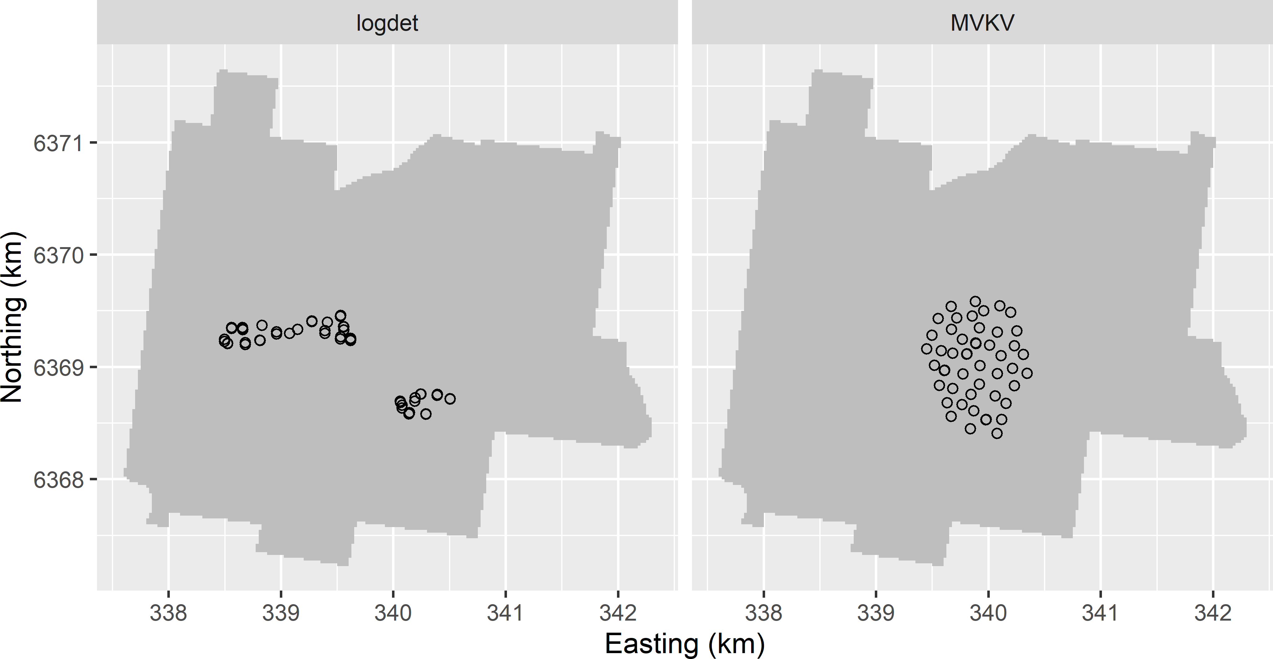
Figure 24.6: Optimised sampling pattern of 100 points for semivariogram estimation, using the log of the determinant of the inverse Fisher information matrix of the semivariogram parameters (logdet) and the mean estimation variance of the kriging variance (MVKV) as a minimisation criterion.
Both methods for sample optimisation rely, amongst others, on the assumption that the mean and the variance are constant throughout the area. Under this assumption, it is no problem that the sampling units are spatially clustered. So, we assume that the semivariogram estimated from the data collected in a small portion of the study area is representative for the whole study area. If we do not feel comfortable with this assumption, spreading the sampling units throughout the study area by the sampling methods described in the next two sections can be a good option.
Exercises
- Write an R script to design a model-based sample of 50 points for Hunter Valley, to estimate the semivariogram for a study variable. Use logdet as a minimisation criterion. Use as a prior estimate of the semivariogram an exponential model with a distance parameter of 200 m and a ratio of spatial dependence of 0.5. Compare the sample with the optimised sample in Figure 24.6, which was obtained with the same value for the distance parameter and a spatial dependence ratio of 0.8.
- Repeat this for MVKV as a minimisation criterion. Use a spatial coverage sample of 100 points for prediction and a square grid of 200 points for evaluation.
24.4 Optimisation of sampling pattern for semivariogram estimation and mapping
In practice, a reconnaissance survey for semivariogram estimation often is not feasible. A single sample must be designed that is suitable both for estimating the semivariogram parameters and mapping, i.e., prediction with the estimated semivariogram parameters at the nodes of a fine discretisation grid. Another reason is that in a reconnaissance survey we can seldom afford a sample size large enough to obtain reliable estimates of the semivariogram parameters. Papritz et al. (2011) found that for a sample size of 192 points the estimated variance components with balanced and unbalanced nested designs were highly uncertain. For this reason, it is attractive to use also the sampling points designed for spatial prediction (mapping) for estimating the semivariogram. Designing two samples, one for estimation of the semivariogram and one for spatial prediction, is suboptimal. Designing one sample that can be used both for estimation of the semivariogram parameters and for prediction potentially is more efficient.
Finally, with nested sampling and IPP sampling, we aim at estimating the semivariogram of the residuals of a constant mean (see Equation (24.1)). In other words, with these designs we aim at estimating the parameters of a semivariogram model used in ordinary kriging. In situations where we have covariates that can partly explain the spatial variation of the study variable, kriging with an external drift is more appropriate. In these situations, the reconnaissance survey should be tailored to estimating both the regression coefficients associated with the covariates and the parameters of the residual semivariogram.
Model-based methods for designing a single sample for estimation of the model parameters and for prediction with the estimated model parameters are proposed, amongst others, by Zimmerman (2006), Zhu and Stein (2006), Zhu and Zhang (2006), and Marchant and Lark (2007). The methods use a different minimisation criterion. Zimmerman (2006) proposed to minimise the kriging variance (at the centre of a square grid cell) that is augmented by an amount that accounts for the additional uncertainty in the kriging predictions due to uncertainty in the estimated semivariogram parameters, hereafter referred to as the augmented kriging variance (AKV):
\[\begin{equation} AKV(\mathbf{s}_0) = V_\mathrm{OK}(\mathbf{s}_0) + \mathrm{E}[\tau^2(\mathbf{s}_0)]\;, \tag{24.4} \end{equation}\]
with \(V_\mathrm{OK}(\mathbf{s}_0)\) the ordinary kriging variance, see Equation (21.8), and \(\mathrm{E}[\tau^2(\mathbf{s}_0)]\) the expectation of the additional variance component due to uncertainty about the semivariogram parameters estimated by ML. The additional variance component is approximated by a first order Taylor series:
\[\begin{equation} \mathrm{E}[\tau^2(\mathbf{s}_0)]=\sum_{i=1}^p \sum_{j=1}^p \mathrm{Cov}(\theta_i,\theta_j) \frac{\partial \lambda^{\mathrm{T}}} {\partial \theta_i} \mathbf{A}\frac{\partial \lambda} {\partial \theta_j}\;, \tag{24.5} \end{equation}\]
with \(\frac{\partial \lambda} {\partial \theta_j}\) the vector of partial derivatives of the kriging weights with respect to the \(j\)th semivariogram parameter. Comparing Equations (24.5) and (24.3) shows that the two variances differ. VKV quantifies our uncertainty about the estimated kriging variance, whereas \(\mathrm{E}[\tau^2]\) quantifies our uncertainty about the kriging prediction due to uncertainty about the semivariogram parameters. I use the mean of the AKV over the nodes of a prediction grid (evaluation grid) as a minimisation criterion (MAKV). The same criterion can also be used in situations where we have maps of covariates that we want to use in prediction. In that case, the aim is to design a single sample that is used both for estimation of the residual semivariogram and for prediction by kriging with an external drift. The ordinary kriging variance \(V_\mathrm{OK}(\mathbf{s}_0)\) in Equation (24.4) is then replaced by the prediction error variance with kriging with an external drift \(V_\mathrm{KED}(\mathbf{s}_0)\), see Equation (21.20).
Zhu and Stein (2006) proposed as a minimisation criterion a linear combination of AKV (Equation (24.4)) and VKV (Equation (24.3)), referred to as the estimation adjusted criterion (EAC):
\[\begin{equation} EAC(\mathbf{s}_0) = AKV(\mathbf{s}_0) + \frac{1}{2V_{\mathrm{OK}}(\mathbf{s}_0)} VKV(\mathbf{s}_0)\;. \tag{24.6} \end{equation}\]
Again, the mean of the EAC values (MEAC) over the nodes of a prediction grid (evaluation) is used as a minimisation criterion.
Computing time for optimisation of the coordinates of a large sample, say, \(>50\) points, can become prohibitively long. To reduce computing time, Zhu and Stein (2006) proposed a two-step approach. In the first step, for a fixed proportion \(p \in (0,1)\) the locations of \((1-p)\;n\) points are optimised for prediction with given parameters, for instance by minimising MKV. This ‘prediction sample’ is supplemented with \(p \;n\) points, so that the two combined samples of size \(n\) minimise logdet or MVKV. This is repeated for different values of \(p\). In the second step, MEAC is computed for the combined samples of size \(n\), and the proportion and the associated sample with minimum MEAC are selected.
A simplification of this two-step approach is to select in the first step a square grid or a spatial coverage sample (Section 17.2), and to supplement this sample by a fixed number of points whose coordinates are optimised by spatial simulated annealing (SSA), using either MAKV or MEAC computed from both samples (grid sample or spatial coverage sample plus supplemental sample) as a minimisation criterion. In SSA the grid or spatial coverage sample is fixed, i.e., the locations are not further optimised. Lark and Marchant (2018) recommended as a rule of thumb to add about 10% of the fixed sample as short distance points.
The following code chunks show how the AKV and EAC can be computed. First, a spatial coverage sample of 90 points is selected using function stratify of package spcosa, see Section 17.2. In addition, a simple random sample of 10 points is selected. This sample is the initial supplemental sample, whose locations are optimised. As before, a square grid of 200 points is used as an evaluation sample.
library(spcosa)
set.seed(314)
mystrata <- stratify(grdHunterValley, nStrata = 90, equalArea = FALSE, nTry = 10)
mysample_SC <- as(spsample(mystrata), "SpatialPoints")
nsup <- 10
units <- sample(nrow(grdHunterValley), nsup)
mysample_sup0 <- as(grdHunterValley[units, ], "SpatialPoints")
mysample_eval <- spsample(
  x = grdHunterValley, n = 200, type = "regular", offset = c(0.5, 0.5))
The next step is to compute the inverse of the Fisher information matrix, given a preliminary semivariogram model, which is used as the variance-covariance matrix of the estimated semivariogram parameters. Contrary to Section 24.3 now all sampling locations are used to compute this matrix. The locations of the spatial coverage sample and the supplemental sample are merged into one SpatialPoints object.
To learn how the Fisher information matrix is computed, refer to the code chunks in Section 24.3. The inverse of this matrix can be computed with function solve.
In the next code chunk, for each evaluation point the kriging weights (L), the kriging variance (var), the perturbed kriging weights (pL), and the perturbed kriging variances (pvar) are computed. In the final lines, the partial derivatives of the kriging weights (dL) and the kriging variances (dvar) with respect to the semivariogram parameters are computed. The partial derivatives of the kriging variances with respect to the semivariogram parameters are needed for computing VKV, see Equation (24.3), which in turn is needed for computing criterion EAC, see Equation (24.6).
L <- matrix(nrow = length(mysample_eval), ncol = nobs)
pL <- array(
  dim = c(length(mysample_eval), length(mysample), length(thetas)))
var <- numeric(length = length(mysample_eval))
pvar <- matrix(nrow = length(mysample_eval), ncol = length(thetas))
for (i in seq_len(length(mysample_eval))) {
  b <- c(A0[i, ], 1)
  l <- solve(B, b)
  L[i, ] <- l[1:nobs]
  var[i] <- 1 - l[1:nobs] %*% A0[i, ] - l[-(1:nobs)]
  for (j in seq_len(length(thetas))) {
    pl <- solve(pB[[j]], pb[[j]][i, ])
    pL[i, , j] <- pl[1:nobs]
    pvar[i, j] <- 1 - pl[1:nobs] %*% pA0[[j]][i, ] - pl[-(1:nobs)]
  }
}
dL <- dvar <- list()
for (i in seq_len(length(thetas))) {
  dL[[i]] <- (pL[, , i] - L) / (thetas[i] * perturbation)
  dvar[[i]] <- (pvar[, i] - var) / (thetas[i] * perturbation)
}
In the next code chunk, the expected variance due to uncertainty about the semivariogram parameters (Equation (24.5)) is computed.
tausq <- numeric(length = length(mysample_eval))
tausqk <- 0
for (k in seq_len(length(mysample_eval))) {
  for (i in seq_len(length(dL))) {
    for (j in seq_len(length(dL))) {
      tausqijk <- invI[i, j] * t(dL[[i]][k, ]) %*% A %*% dL[[j]][k, ]
      tausqk <- tausqk + tausqijk
    }
  }
  tausq[k] <- tausqk
  tausqk <- 0
}
The AKVs are computed by adding the kriging variances and the extra variances due to semivariogram uncertainty (Equation (24.4)). The VKV values and the EAC values are computed. Both the AKV and the EAC differ among the evaluation points. As a summary, the mean of the two variables is computed.
augmentedvar <- var + tausq
MAKV0 <- mean(augmentedvar)
VKV <- numeric(length = length(var))
for (i in seq_len(length(dvar))) {
  for (j in seq_len(length(dvar))) {
    VKVij <- invI[i, j] * dvar[[i]] * dvar[[j]]
    VKV <- VKV + VKVij
  }
}
EAC <- augmentedvar + (VKV / (2 * var))
MEAC0 <- mean(EAC)
For the spatial coverage sample of 90 points supplemented by a simple random sample of 10 points, MAKV equals 0.849 and MEAC equals 0.890.
The sample can be optimised with spsann function optimUSER. Argument points is a list containing a data frame, or matrix, with the coordinates of the fixed points (assigned to subargument fixed) and an integer of the number of supplemental points of which the locations are optimised (assigned to sub-argument free). As already stressed above, an important difference with Section 24.3 is that the free and the fixed sample are merged and used together both for estimation of the semivariogram and for prediction. The objective functions MAKV and MEAC are defined in package sswr. Computing time for minimisation of MAKV was 28.16 minutes and of MEAC 28.88 minutes.
candi <- spsample(grdHunterValley, type = "regular",
                  cellsize = c(50, 50), offset = c(0.5, 0.5))
candi <- as.data.frame(candi)
names(candi) <- c("x", "y")
schedule <- scheduleSPSANN(
  initial.acceptance = c(0.8, 0.95),
  initial.temperature = 0.008, temperature.decrease = 0.8,
  chains = 300, chain.length = 10, stopping = 10,
  x.min = 0, y.min = 0, cellsize = 50)
fixed <- coordinates(mysample_SC)
names(fixed) <- c("x", "y")
pnts <- list(fixed = fixed, free = nsup)
set.seed(314)
res <- optimUSER(
  points = pnts, candi = candi,
  fun = MAKV,
  esample = mysample_eval,
  model = "Exp", thetas = thetas, perturbation = 0.01,
  schedule = schedule, track = TRUE)
Figure 24.7 shows for Hunter Valley a spatial coverage sample of 90 points, supplemented by 10 points optimised by SSA, using MAKV and MEAC as a minimisation criterion.
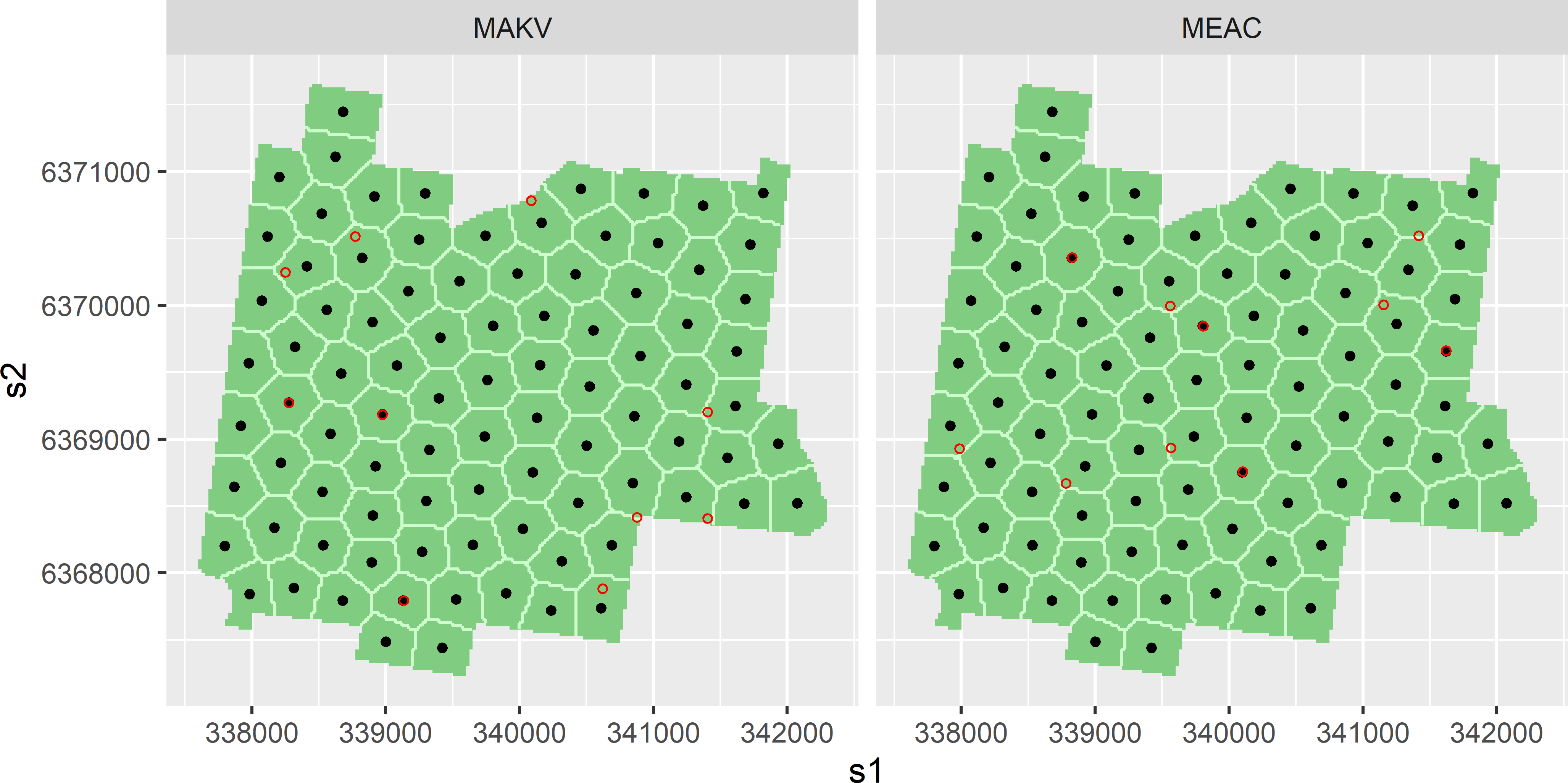
Figure 24.7: Optimised sampling pattern of 10 points supplemented to spatial coverage sample of 90 points, for semivariogram estimation and prediction, using the mean augmented kriging variance (MAKV) and the mean estimation adjusted criterion (MEAC) as a minimisation criterion. The prior semivariogram used in optimising the sampling pattern of the supplemental sample is an exponential semivariogram with a range of 200 m and a ratio of spatial dependence of 0.5.
The frequency distribution of the shortest distance to the spatial coverage sample is shown in Figure 24.8. With both criteria there are several supplemental points at very short distance of a point of the spatial coverage sample. The remaining points are at large distances of spatial coverage sample points. The average distance between neighbouring spatial coverage sampling points equals 381 m.
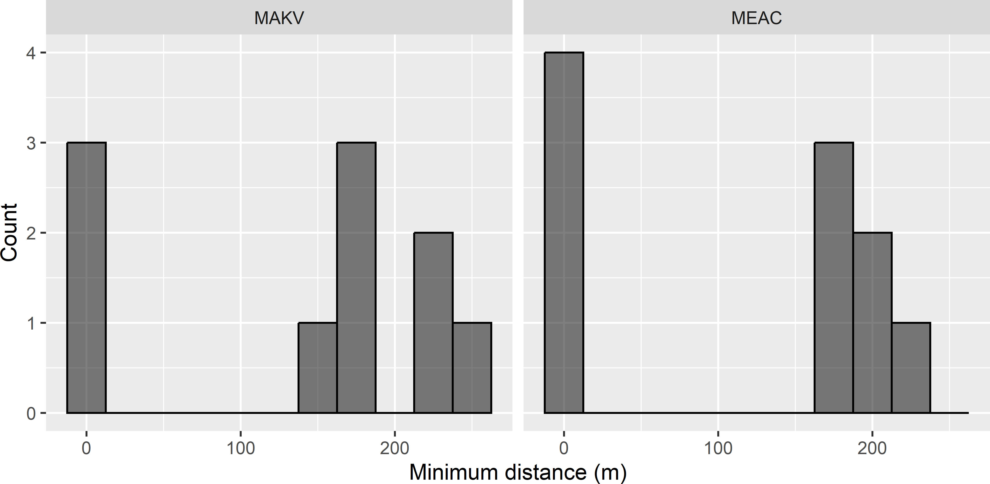
Figure 24.8: Frequency distributions of the shortest distance to the spatial coverage sample of the supplemental sample, optimised with the mean augmented kriging variance (MAKV) and the mean estimation adjusted criterion (MEAC).
MAKV of the optimised sample equals 0.795 which is 94% of MAKV of the initial sample. MEAC of the optimised sample equals 0.808 which is 91% of MEAC of the initial sample. The reduction of these two criteria through the optimisation is much smaller than for logdet and MVKV in Section 24.3. This can be explained by the small number of sampling units that is optimised: only the locations of 10 points are optimised, 90 are fixed. In Section 24.3 all 100 locations were optimised.
Exercises
- Write an R script to select from Hunter Valley a spatial coverage sample of 80 points supplemented by 20 points. Use MEAC as a minimisation criterion, an exponential semivariogram with a distance parameter of 200 m and a ratio of spatial dependence of 0.8. Compare the minimised MEAC with MEAC reported above, obtained by supplementing a spatial coverage sample of 90 points by 10 points.
24.5 A practical solution
Based on the optimised samples shown above, a straightforward, simple sampling design for estimation of the model parameters and for prediction is a spatial coverage sample supplemented with randomly selected points between the points of the spatial coverage sample at some chosen fixed distances. Figure 24.9 shows an example. A simple random subsample without replacement of size 10 is selected from the 90 points of the spatial coverage sample. These points are used as starting points to select a point at a distance of 20 m in a random direction.
h <- 20
m <- 10
set.seed(314)
units <- sample(nrow(mysample_SC), m, replace = FALSE)
mySCsubsample <- mysample_SC[units, ]
dxy <- matrix(nrow = m, ncol = 2)
angle <- runif(n = m, min = 0, max = 2 * pi)
dxy[, 1] <- h * sin(angle); dxy[, 2] <- h * cos(angle)
mysupsample <- mySCsubsample + dxy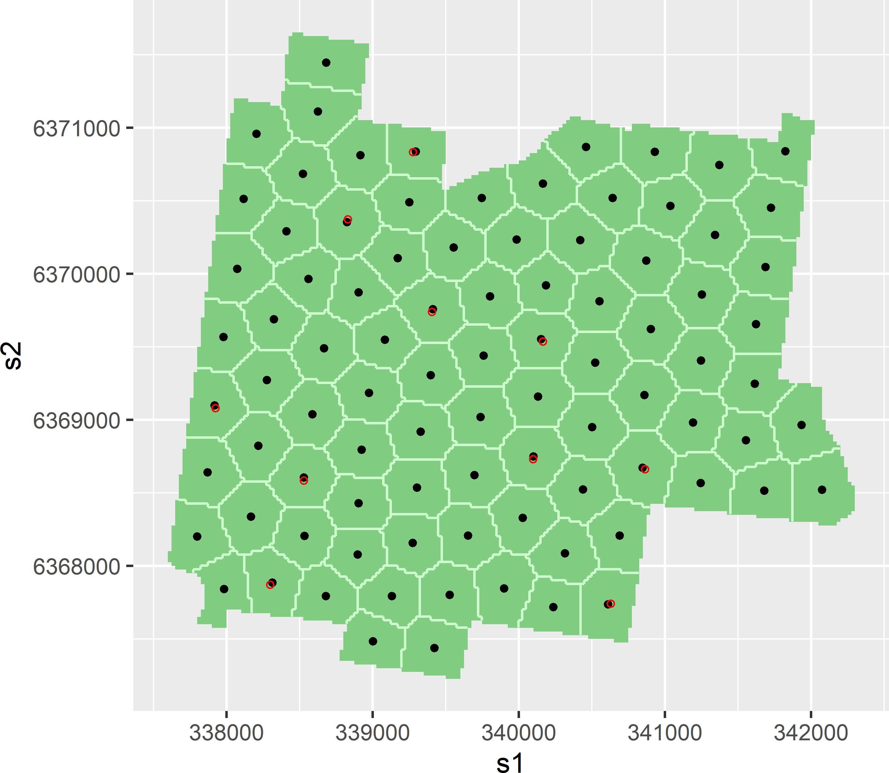
Figure 24.9: Spatial coverage sample of 90 points supplemented by 10 points at short distance (20 m) from randomly selected spatial coverage points.
MAKV of this sample equals 0.808, and MEAC equals 0.816. For MAKV, 25% of the maximal reduction is realised by this practical solution; for MEAC, this is 10%.