Chapter 3 Simple random sampling

Simple random sampling is the most basic form of probability sampling. There are two subtypes:

1. simple random sampling with replacement; and
2. simple random sampling without replacement.

This distinction is irrelevant for infinite populations. In sampling with replacement a population unit may be selected more than once.

In R a simple random sample can be selected with or without replacement by function sample from the base package. For instance, a simple random sample without replacement of 10 units from a population of 100 units labelled as \(1,2, \dots ,100\), can be selected by

sample(100, size = 10, replace = FALSE)

 [1]  21   7   5  16  58  76  44 100  71  84

The number of units in the sample is referred to as the sample size (\(n = 10\) in the code chunk above). Use argument replace = TRUE to select a simple random sample with replacement.

When the spatial population is continuous and infinite, as in sampling points from an area, the infinite population is discretised by a very fine grid. Discretisation is not strictly needed (we could also select points directly), but it is used in this book for reasons explained in Chapter 1. The centres of the grid cells are then listed in a data frame, which serves as the sampling frame (Chapter 1). In the next code chunk, a simple random sample without replacement of size 40 is selected from Voorst. The infinite population is represented by the centres of square grid cells with a side length of 25 m. These centres are listed in tibble¹ grdVoorst.

n <- 40
N <- nrow(grdVoorst)
set.seed(314)
units <- sample(N, size = n, replace = FALSE)
mysample <- grdVoorst[units, ]
mysample

# A tibble: 40 x 4
       s1      s2     z stratum
    <dbl>   <dbl> <dbl> <chr>  
 1 206992 464506.  23.5 EA     
 2 202567 464606. 321.  XF     
 3 205092 464530. 124.  XF     
 4 203367 464556.  53.6 EA     
 5 205592 465180.  38.4 PA     
 6 201842 464956. 159.  XF     
 7 201667 464930. 139.  XF     
 8 204317 465306.  59.4 PA     
 9 203042 464406.  90.5 BA     
10 204567 464530.  48.1 PA     
# i 30 more rows

The result of function sample is a vector with the centres of the selected cells of the discretisation grid, referred to as discretisation points. The order of the elements of the vector is the order in which these are selected. Restricting the sampling points to the discretisation points can be avoided as follows. A simple random sample of points is selected in two stages. First, n times a grid cell is selected by simple random sampling with replacement. Second, every time a grid cell is selected, one point is selected fully randomly from that grid cell. This selection procedure accounts for the infinite number of points in the population. In the code chunk below, the second step of this selection procedure is implemented with function jitter. It adds random noise to the spatial coordinates of the centres of the selected grid cells, by drawing from a continuous uniform distribution \(\text{unif}(-c,c)\), with \(c\) half the side length of the square grid cells. With this selection procedure we respect that the population actually is infinite.

set.seed(314)
units <- sample(N, size = n, replace = TRUE)
mysample <- grdVoorst[units, ]
cellsize <- 25
mysample$s1 <- jitter(mysample$s1, amount = cellsize / 2)
mysample$s2 <- jitter(mysample$s2, amount = cellsize / 2)
mysample

# A tibble: 40 x 4
        s1      s2     z stratum
     <dbl>   <dbl> <dbl> <chr>  
 1 206986. 464493.  23.5 EA     
 2 202574. 464609. 321.  XF     
 3 205095. 464527. 124.  XF     
 4 203369. 464556.  53.6 EA     
 5 205598. 465181.  38.4 PA     
 6 201836. 464965. 159.  XF     
 7 201665. 464941. 139.  XF     
 8 204319. 465310.  59.4 PA     
 9 203052. 464402.  90.5 BA     
10 204564. 464529.  48.1 PA     
# i 30 more rows

Variable stratum is not used in this chapter but in the next chapter. The selected sample is shown in Figure 3.1.

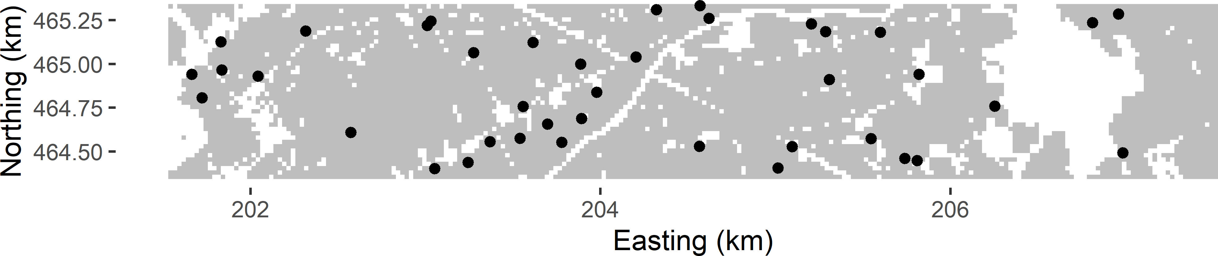
Figure 3.1: Simple random sample of size 40 from Voorst.

Dropouts

In practice, it may happen that inspection in the field shows that a selected sampling unit does not belong to the target population or cannot be observed for whatever reason (e.g., no permission). For instance, in a soil survey the sampling unit may happen to fall on a road or in a built-up area. What to do with these dropouts? Shifting this unit to a nearby unit may lead to a biased estimator of the population mean, i.e., a systematic error in the estimated population mean. Besides, knowledge of the inclusion probabilities is lost. This can be avoided by discarding these units and replacing them by sampling units from a back-up list, selected in the same way, i.e., by the same type of sampling design. The order of sampling units in this list must be the order in which they are selected. In summary, do not replace a deleted sampling unit by the nearest sampling unit from the back-up list, but by the first unit, not yet selected, from the back-up list.

3.1 Estimation of population parameters

In simple random sampling without replacement of a finite population, every possible sample of \(n\) units has an equal probability of being selected. There are \(\binom{N}{n}\) samples of size \(n\) and \(\binom{N-1}{n-1}\) samples that contain unit \(k\). From this it follows that the probability that unit \(k\) is included in the sample is \(\binom{N-1}{n-1}/\binom{N}{n}=\frac{n}{N}\) (Lohr 1999). Substituting this in the general \(\pi\) estimator for the total (Equation (2.2)) gives for simple random sampling without replacement (from finite populations)

\[\begin{equation} \hat{t}(z)=\frac{N}{n}\sum_{k \in \mathcal{S}} z_k = N \bar{z}_{\mathcal{S}} \;, \tag{3.1} \end{equation}\]

with \(\bar{z}_{\mathcal{S}}\) the unweighted sample mean. So, for simple random sampling without replacement the \(\pi\) estimator of the population mean is the unweighted sample mean:

\[\begin{equation} \hat{\bar{z}} = \bar{z}_{\mathcal{S}} = \frac{1}{n}\sum_{k \in \mathcal{S}} z_k \;. \tag{3.2} \end{equation}\]

In simple random sampling with replacement of finite populations, a unit may occur multiple times in the sample \(\mathcal{S}\). In this case, the population total can be estimated by the pwr estimator (Särndal, Swensson, and Wretman 1992)

\[\begin{equation} \hat{t}(z)= \frac{1}{n} \sum_{k \in \mathcal{S}} \frac{z_{k}}{p_{k}} \;, \tag{3.3} \end{equation}\]

where \(n\) is the number of draws (sample size) and \(p_{k}\) is the draw-by-draw selection probability of unit \(k\). With simple random sampling \(p_{k}=1/N, k=1, \dots , N\). Inserting this in the pwr estimator yields

\[\begin{equation} \hat{t}(z)= \frac{N}{n} \sum_{k \in \mathcal{S}} z_{k} \;, \tag{3.4} \end{equation}\]

which is equal to the \(\pi\) estimator of the population total for simple random sampling without replacement.

Alternatively, the population total can be estimated by the \(\pi\) estimator. With simple random sampling with replacement the inclusion probability of each unit \(k\) equals \(1-\left(1-\frac{1}{N}\right)^n\), which is smaller than the inclusion probability with simple random sampling without replacement of size \(n\) (Särndal, Swensson, and Wretman 1992). Inserting these inclusion probabilities in the general \(\pi\) estimator of the population total (Equation (2.2)), where the sample \(\mathcal{S}\) is reduced to the unique units in the sample, yields the \(\pi\) estimator of the total for simple random sampling with replacement.

With simple random sampling of infinite populations, the \(\pi\) estimator of the population mean equals the sample mean. Multiplying this estimator with the area of the region of interest \(A\) yields the \(\pi\) estimator of the population total:

\[\begin{equation} \hat{t}(z)= \frac{A}{n}\sum_{k \in \mathcal{S}}z_{k} \;. \tag{3.5} \end{equation}\]

As explained above, selected sampling units that do not belong to the target population must be replaced by a unit from a back-up list if we want to observe the intended number of units. The question then is how to estimate the population total and mean. We cannot use the \(\pi\) estimator of Equation (3.1) to estimate the population total, because we do not know the population size \(N\). The population size can be estimated by

\[\begin{equation} \widehat{N} = \frac{n-d}{n}N^*\;, \end{equation}\]

with \(d\) the number of dropouts and \(N^*\) the supposed population size, i.e., the number of units in the sampling frame used to select the sample. This yields the inclusion probability

\[\begin{equation} \pi_k = \frac{n}{\widehat{N}}=\frac{n^2}{(n-d)N^*}\;. \end{equation}\]

Inserting this in the \(\pi\) estimator of the population total yields

\[\begin{equation} \hat{t}(z) = \frac{(n-d)N^*}{n^2}\sum_{k \in \mathcal{S}} z_{k} = \frac{(n-d)N^*}{n} \bar{z}_{\mathcal{S}}=\widehat{N}\bar{z}_{\mathcal{S}}\;. \end{equation}\]

A natural estimator of the population mean is

\[\begin{equation} \hat{\bar{z}} = \frac{\hat{t}(z)}{\widehat{N}}=\bar{z}_{\mathcal{S}}\;. \end{equation}\]

This estimator is a so-called ratio estimator: both the numerator and denominator are estimators of totals. See Section 10.2 for more information about this estimator.

The simple random sample of size 40 selected above is used to estimate the total mass of soil organic matter (SOM) in the population. First, the population mean is estimated.

mz <- mean(mysample$z)

The estimated mean SOM concentration is 93.3 g kg^-1. Simply multiplying the estimated mean by the area \(A\) to obtain an estimate of the population total is not very useful, as the dimension of the total then is in g kg^-1 m². To estimate the total mass of SOM in the soil layer \(0-30\) cm, first the soil volume in m³ is computed by the total number of grid cells, \(N\), multiplied by the size of the grid cells and by the thickness of the soil layer. The total is then estimated by the product of this volume, the bulk density of soil (1,500 kg m^-3), and the estimated population mean (g kg^-1). This is multiplied by 10^-6 to obtain the total mass of SOM in Mg (1 Mg is 1,000 kg).

vol_soil <- N * 25^2 * 0.3
bd <- 1500
tz <- vol_soil * bd * mz * 10^-6

The estimated total is 197,545 Mg (420 Mg ha^-1).

Note that a constant bulk density is used. Ideally, this bulk density is also measured at the sampling points, by collecting soil aliquots of a constant volume. The measured SOM concentration and bulk density can then be used to compute the volumetric SOM concentration in kg m^-3 at the sampling points. The estimated population mean of this volumetric SOM concentration can then be multiplied by the total volume of soil in the study area, to get an estimate of the total mass of SOM in the study area.

The simulated population is now sampled 10,000 times to see how sampling affects the estimates. For each sample, the population mean is estimated by the sample mean. Figure 3.2 shows the approximated sampling distribution of the \(\pi\) estimator of the mean SOM concentration. Note that the sampling distribution is nearly symmetric, whereas the frequency distribution of the SOM concentrations in the population is far from symmetric, see Figure 1.4. The increased symmetry is due to the averaging of 40 numbers.

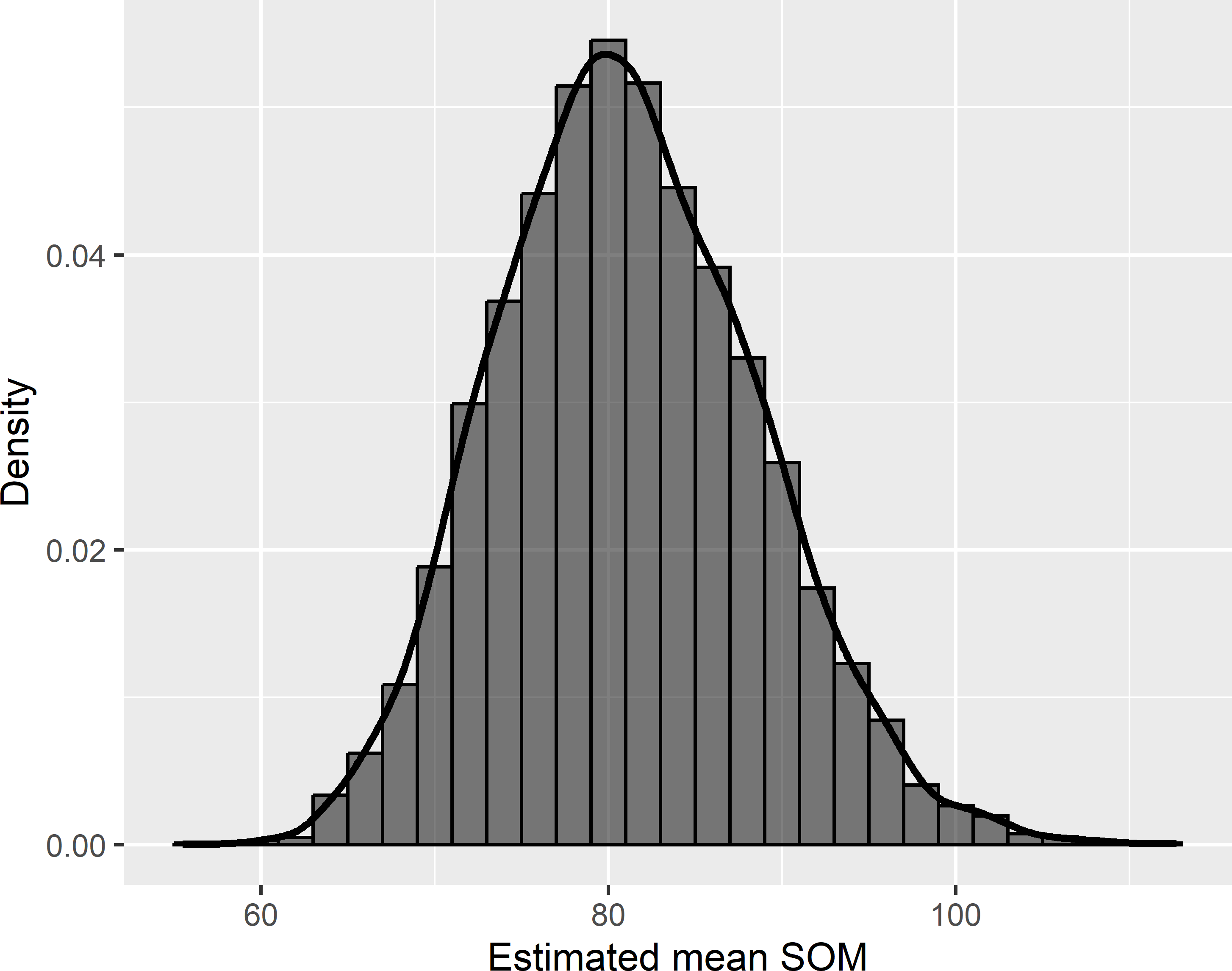
Figure 3.2: Approximated sampling distribution of the \(\pi\) estimator of the mean SOM concentration (g kg^-1) in Voorst for simple random sampling of size 40.

If we would repeat the sampling an infinite number of times and make the width of the bins in the histogram infinitely small, then we obtain, after scaling so that the sum of the area under the curve equals 1, the sampling distribution of the estimator of the population mean. Important summary statistics of this sampling distribution are the expectation (mean) and the variance.

When the expectation equals the population mean, there is no systematic error. The estimator is then said to be design-unbiased. In Chapter 21 another type of unbiasedness is introduced, model-unbiasedness. The difference between design-unbiasedness and model-unbiasedness is explained in Chapter 26. In following chapters of Part I unbiased means design-unbiased. Actually, it is not the estimator which is unbiased, but the combination of a sampling design and an estimator. For instance, with an equal probability sampling design, the sample mean is an unbiased estimator of the population mean, whereas it is a biased estimator in combination with an unequal probability sampling design.

The variance, referred to as the sampling variance, is a measure of the random error. Ideally, this variance is as small as possible, so that there is a large probability that for an individual estimate the estimation error is small. The variance is a measure of the precision of an estimator. An estimator with a small variance but a strong bias is not a good estimator. To assess the quality of an estimator, we should look at both. The variance and the bias are often combined in the mean squared error (MSE), which is the sum of the variance and the squared bias. An estimator with a small MSE is an accurate estimator. So, contrary to precision, accuracy also accounts for the bias.

Do not confuse the population variance and the sampling variance. The population variance, or spatial variance, is a population characteristic, whereas the sampling variance is a characteristic of a sampling strategy, i.e., a combination of a sampling design and an estimator. The sampling variance quantifies our uncertainty about the population mean. The sampling variance can be manipulated by changing the sample size \(n\), the type of sampling design, and the estimator. This has no effect on the population variance. The average of the 10,000 estimated population means equals 81.1 g kg^-1, so the difference with the true population mean equals -0.03 g kg^-1. The variance of the 10,000 estimated population means equals 55.8 (g kg^-1)². The square root of this variance, referred to as the standard error, equals 7.47 g kg^-1. Note that the standard error has the same units as the study variable, g kg^-1, whereas the units of the variance are the squared units of the study variable.

3.1.1 Population proportion

In some cases one is interested in the proportion of the population (study area) satisfying a given condition. Think, for instance, of the proportion of trees in a forest infected by some disease, the proportion of an area or areal fraction, in which a soil pollutant exceeds some critical threshold, or the proportion of an area where habitat conditions are suitable for some endangered species. Recall that a population proportion is defined as the population mean of an 0/1 indicator \(y\) with value 1 if the condition is satisfied, and 0 otherwise (Subsection 1.1.1). For simple random sampling, this population proportion can be estimated by the same formula as for the mean (Equation (3.2)):

\[\begin{equation} \hat{p} = \frac{1}{n}\sum_{k \in \mathcal{S}} y_k \;. \tag{3.6} \end{equation}\]

3.1.2 Cumulative distribution function and quantiles

The population cumulative distribution function (CDF) is defined in Equation (1.4). A population CDF can be estimated by repeated application of the indicator technique described in the previous subsection on estimating a population proportion. A series of threshold values is chosen. Each threshold results in \(n\) indicator values having value 1 if the observed study variable \(z\) of unit \(k\) is smaller than or equal to the threshold, and 0 otherwise. These indicator values are then used to estimate the proportion of the population with a \(z\)-value smaller than or equal to that threshold. For simple random sampling, these proportions can be estimated with Equation (3.6). Commonly, the unique \(z\)-values in the sample are used as threshold values, leading to as many estimated population proportions as there are unique values in the sample.

Figure 3.3 shows the estimated CDF, estimated from the simple random sample of 40 units from Voorst. The steps are at the unique values of SOM in the sample.

ggplot(mysample, mapping = aes(z)) +
  stat_ecdf(geom = "step") +
  scale_x_continuous(name = "SOM") +
  scale_y_continuous(name = "F")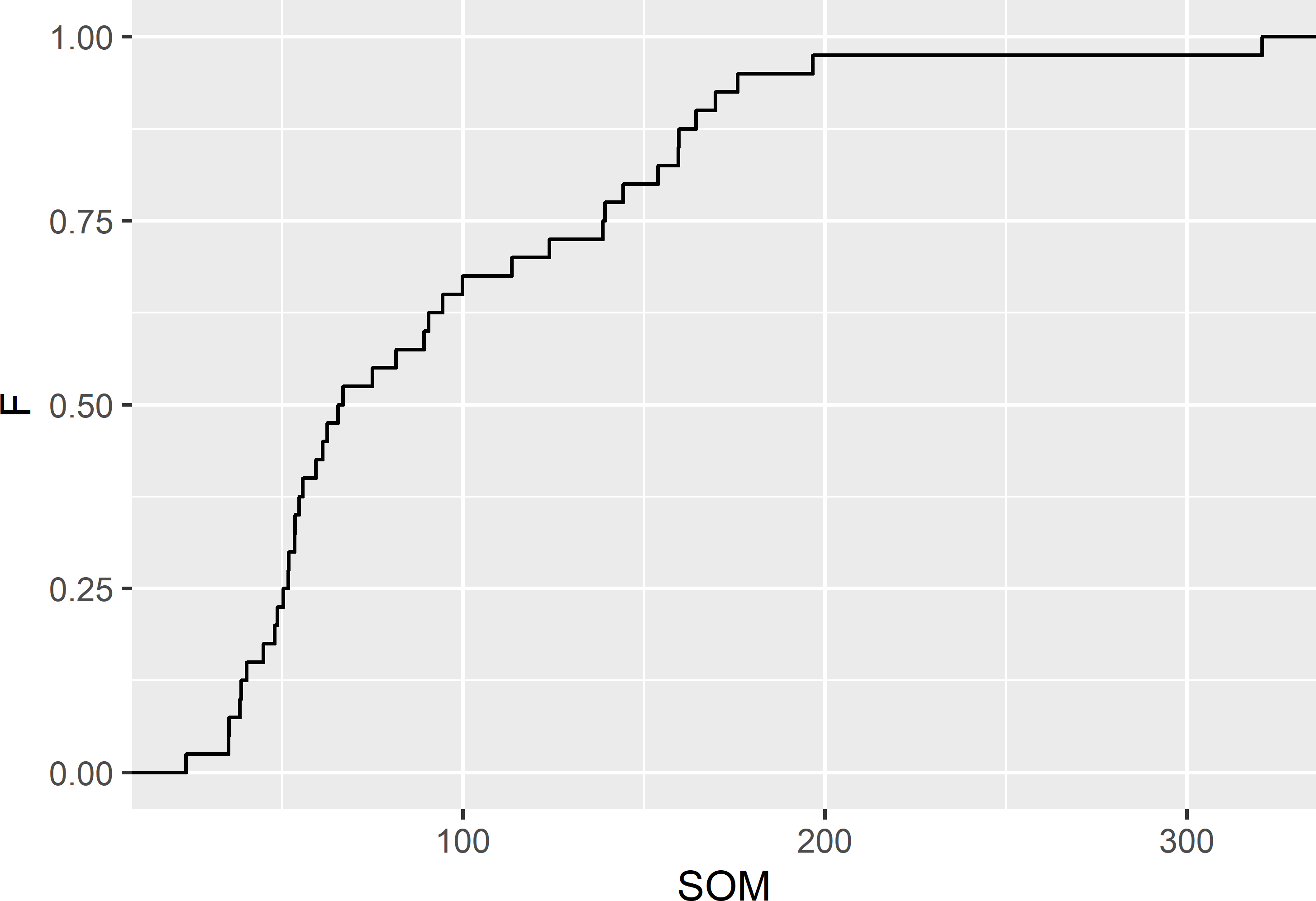

Figure 3.3: Cumulative distribution function of the SOM concentration (g kg^-1) in Voorst, estimated from the simple random sample of 40 units.

The estimated population proportions can be used to estimate a population quantile for any population proportion (cumulative frequency, probability), for instance the median, first quartile, and third quartile, corresponding to a population proportion of 0.5, 0.25, and 0.75, respectively. A simple estimator is the smallest \(k\)th order statistic with an estimated proportion larger than or equal to the desired cumulative frequency (Hyndman and Fan 1996).

The estimated CDF shows jumps of size \(1/n\), so that the estimated population proportion can be larger than the desired proportion. The estimated population proportions therefore are often interpolated, for instance linearly. Function quantile of the stats package can be used to estimate a quantile. With argument type = 4 linear interpolation is used to estimate the quantiles.

Function quantile actually computes sample quantiles, i.e., it assumes that the population units are selected with equal inclusion probabilities (as in simple random sampling), so that the estimators of the population proportions obtained with Equation (3.6) are unbiased. With unequal inclusion probabilities these probabilities must be accounted for in estimating the population proportions, see following chapters.

quantile(mysample$z, probs = c(0.25, 0.5, 0.75), type = 4) %>%
  round(1)

  25%   50%   75% 
 50.4  65.6 138.7 

Note the pipe operator %>% of package magrittr (Bache and Wickham 2020) forwarding the result of function quantile to function round.

Package QuantileNPCI (N. Hutson, Hutson, and Yan 2019) can be used to compute a non-parametric confidence interval estimate of a quantile, using fractional order statistics (A. D. Hutson 1999). Parameter q specifies the proportion.

library(QuantileNPCI)
res <- quantCI(mysample$z, q = 0.5, alpha = 0.05, method = "exact")

The estimated median equals 66.2 g kg^-1, the lower bound of the 95% confidence interval equals 54.0 g kg^-1, and the upper bound equals 98.1 g kg^-1.

Exercises

1. Compare the approximated sampling distribution of the \(\pi\) estimator of the mean SOM concentration of Voorst (Figure 3.2) with the histogram of the 7,528 simulated SOM values (Figure 1.4). Explain the differences.
   
2. What happens with the spread in the approximated sampling distribution (variance of estimated population means) when the sample size \(n\) is increased?
   
3. Suppose we would repeat the sampling \(10^{12}\) number of times, what would happen with the difference between the average of the estimated population means and the true population mean?

3.2 Sampling variance of estimator of population parameters

For simple random sampling of an infinite population and simple random sampling with replacement of a finite population, the sampling variance of the estimator of the population mean equals

\[\begin{equation} V\!\left(\hat{\bar{z}}\right)=\frac{S^{2}(z)}{n} \;, \tag{3.7} \end{equation}\]

with \(S^{2}(z)\) the population variance, also referred to as the spatial variance. For finite populations, this population variance is defined as (Lohr 1999)

\[\begin{equation} S^{2}(z)=\frac{1}{N-1}\sum\limits_{k=1}^N\left(z_{k}-\bar{z}\right)^{2} \;, \tag{3.8} \end{equation}\]

and for infinite populations as

\[\begin{equation} S^{2}(z) = \frac{1}{A} \int \limits_{\mathbf{s} \in \mathcal{A}} \left(z(\mathbf{s})-\bar{z}\right)^2\text{d}\mathbf{s} \;, \tag{3.9} \end{equation}\]

with \(z(\mathbf{s})\) the value of the study variable \(z\) at a point with two-dimensional coordinates \(\mathbf{s}=(s_1,s_2)\), \(A\) the area of the study area, and \(\mathcal{A}\) the study area. In practice, we select only one sample, i.e., we do not repeat the sampling many times. Still it is possible to estimate the variance of the estimator of the population mean if we would repeat the sampling. In other words, we can estimate the sampling variance of the estimator of the population mean from a single sample. We do so by estimating the population variance from the sample, and this estimate can then be used to estimate the sampling variance of the estimator of the population mean. For simple random sampling with replacement from finite populations, the sampling variance of the estimator of the population mean can be estimated by

\[\begin{equation} \widehat{V}\!\left(\hat{\bar{z}}\right)=\frac{\widehat{S^2}(z)}{n}= \frac{1}{n\,(n-1)}\sum\limits_{k \in \mathcal{S}}\left(z_{k}-\bar{z}_{\mathcal{S}}\right)^{2} \;, \tag{3.10} \end{equation}\]

with \(\widehat{S^2}(z)\) the estimated population variance. With simple random sampling, the sample variance, i.e., the variance of the sample data, is an unbiased estimator of the population variance. The variance estimator of Equation (3.10) can also be used for infinite populations. For simple random sampling without replacement from finite populations, the sampling variance of the estimator of the population mean can be estimated by

\[\begin{equation} \widehat{V}\!\left(\hat{\bar{z}}\right)=\left(1-\frac{n}{N}\right)\frac{\widehat{S^2}(z)}{n} \;. \tag{3.11} \end{equation}\]

The term \(1-\frac{n}{N}\) is referred to as the finite population correction (fpc).

In the sampling experiment described above, the average of the 10,000 estimated sampling variances equals 55.7 (g kg^-1)². The true sampling variance equals 55.4 (g kg^-1)². So, the difference is very small, indicating that the estimator of the sampling variance, Equation (3.11), is design-unbiased.

The sampling variance of the estimator of the total of a finite population can be estimated by multiplying the estimated variance of the estimator of the population mean by \(N^2\). For simple random sampling without replacement this estimator thus equals

\[\begin{equation} \widehat{V}\!\left(\hat{t}(z)\right)=N^2 \left(1-\frac{n}{N}\right)\frac{\widehat{S^{2}}(z)}{n} \;. \tag{3.12} \end{equation}\]

For simple random sampling of infinite populations, the sampling variance of the estimator of the total can be estimated by

\[\begin{equation} \widehat{V}\!\left(\hat{t}(z)\right)=A^2\frac{\widehat{S^{2}}(z)}{n} \;. \tag{3.13} \end{equation}\]

The sampling variance of the estimator of a proportion \(\hat{p}\) for simple random sampling without replacement of a finite population can be estimated by

\[\begin{equation} \widehat{V}\!\left(\hat{p}\right)=\left( 1-\frac{n}{N}\right) \frac{\hat{p}(1-\hat{p})}{n-1} \;. \tag{3.14} \end{equation}\]

The numerator in this estimator is an estimate of the population variance of the indicator. Note that this estimated population variance is divided by \(n-1\), and not by \(n\) as in the estimator of the population mean (Lohr 1999).

Estimation of the standard error of the estimated population mean in R is very straightforward. To estimate the standard error of the estimated total in Mg, the standard error of the estimated population mean must be multiplied by a constant equal to the product of the soil volume, the bulk density, and \(10^{-6}\); see second code chunk in Section 3.1.

se_mz <- sqrt(var(mysample$z) / n)
se_tz <- se_mz * vol_soil * bd * 10^-6

The estimated standard error of the estimated total equals 20,334 Mg. This standard error does not account for spatial variation of bulk density.

Although there is no advantage in using package survey (Lumley 2021) to compute the \(\pi\) estimator and its standard error for this simple sampling design, I illustrate how this works. For more complex designs and alternative estimators, estimation of the population mean and its standard error with functions defined in this package is very convenient, as will be shown in the following chapters.

First, the sampling design that is used to select the sampling units is specified with function svydesign. The first argument specifies the sampling units. In this case, the centres of the discretisation grid cells are used as sampling units, which is indicated by the formula id = ~ 1. In Chapter 6 clusters of population units are used as sampling units, and in Chapter 7 both clusters and individual units are used as sampling units. Argument probs specifies the inclusion probabilities of the sampling units. Alternatively, we may specify the weights with argument weights, which are in this case equal to the inverse of the inclusion probabilities. Variable pi is a column in tibble mysample, which is indicated with the tilde in probs = ~ pi.

The population mean is then estimated with function svymean. The first argument is a formula specifying the study variable. Argument design specifies the sampling design.

library(survey)
mysample$pi <- n / N
design_si <- svydesign(id = ~ 1, probs = ~ pi, data = mysample)
svymean(~ z, design = design_si)

    mean     SE
z 93.303 9.6041

For simple random sampling of finite populations without replacement, argument fpc is used to correct the standard error.

mysample$N <- N
design_si_fp <- svydesign(id = ~ 1, probs = ~ pi, fpc = ~ N, data = mysample)
svymean(~ z, design_si_fp)

    mean     SE
z 93.303 9.5786

The estimated standard error is smaller now due to the finite population correction, see Equation (3.11).

Population totals can be estimated with function svytotal, quantiles with function svyquantile, and ratios of population totals with svyratio, to mention a few functions that will be used in following chapters.

svyquantile(~ z, design_si, quantile = c(0.5, 0.9))

$z
     quantile    ci.2.5   ci.97.5       se
0.5  65.56675  53.67764  99.93484 11.43457
0.9 164.36975 153.86258 320.74887 41.25353

attr(,"hasci")
[1] TRUE
attr(,"class")
[1] "newsvyquantile"

Exercises

4. Is the sampling variance for simple random sampling without replacement larger or smaller than for simple random sampling with replacement, given the sample size \(n\)? Explain your answer.
   
5. What is the effect of the population size \(N\) on this difference?
   
6. In Section 3.2 the true sampling variance is reported, i.e., the variance of the estimator of the population mean if we would repeat the sampling an infinite number of times. How can this true sampling variance be computed?
   
7. In reality, we cannot compute the true sampling variance. Why not?

3.3 Confidence interval estimate

A second way of expressing our uncertainty about the estimated total, mean, or proportion is to present not merely a single number, but an interval. The wider the interval, the more uncertain we are about the estimate, and vice versa, the narrower the interval, the more confident we are. To learn how to compute a confidence interval, I return to the sampling distribution of the estimator of the mean SOM concentration. Suppose we would like to compute the bounds of an interval \([a,b]\) such that 5% of the estimated population means is smaller than \(a\), and 5% is larger than \(b\). To compute the lower bound \(a\) and the upper bound \(b\) of this 90% interval, we must specify the distribution function. When the distribution of the study variable \(z\) is normal and we know the variance of \(z\) in the population, then the sampling distribution of the estimator of the population mean is also normal, regardless of the sample size. The larger the sample size, the smaller the effect of the distribution of \(z\) on the sampling distribution of the estimator of the population mean. For instance, even when the distribution of \(z\) is far from symmetric, then still the sampling distribution of the estimator of the population mean is approximately normal if the sample size is large, say \(n > 100\). This is the essence of the central limit theorem. Above, we already noticed that the sampling distribution is much less asymmetric than the frequency distribution of the simulated values, and looks much more like a normal distribution. Assuming a normal distribution, the bounds of the 90% interval are given by

\[\begin{equation} \hat{\bar{z}} \pm u_{(0.10/2)}\cdot \sqrt{V\!\left(\hat{\bar{z}}\right)} \;, \tag{3.15} \end{equation}\]

where \(u_{(0.10/2)}\) is the \(0.95\) quantile of the standard normal distribution, i.e., the value of \(u\) having a tail area of 0.05 to its right. Note that in this equation the sampling variance of the estimator of the population mean \(V\!\left(\hat{\bar{z}}\right)\) is used. In practice, this variance is unknown, because the population variance is unknown, and must be estimated from the sample (Equations (3.10) and (3.11)). To account for the unknown sampling variance, the standard normal distribution is replaced by Student’s t distribution (hereafter shortly referred to as the t distribution), which has thicker tails than the standard normal distribution. This leads to the following bounds of the \(100(1-\alpha)\%\) confidence interval estimate of the mean:

\[\begin{equation} \hat{\bar{z}} \pm t^{(n-1)}_{\alpha /2}\cdot \sqrt{\widehat{V}\!\left(\hat{\bar{z}}\right)} \;, \tag{3.16} \end{equation}\]

where \(t^{(n-1)}_{\alpha /2}\) is the \((1-\alpha /2)\) quantile of the t distribution with \((n-1)\) degrees of freedom. The quantity \((1-\alpha)\) is referred to as the confidence level. The larger the number of degrees of freedom \((n-1)\), the closer the t distribution is to the standard normal distribution. The quantity \(t^{(n-1)}_{1-\alpha /2}\cdot \sqrt{\widehat{V}\!\left(\hat{\bar{z}}\right)}\) is referred to as the margin of error.

Function qt computes a quantile of a t distribution, given the degrees of freedom and the cumulative probability. The bounds of the confidence interval can then be computed as follows.

alpha <- 0.05
margin <- qt(1 - alpha / 2, n - 1, lower.tail = TRUE) * se_mz
lower <- mz - margin
upper <- mz + margin

More easily, we can use method confint of package survey to compute the confidence interval.

confint(svymean(~ z, design_si), df = degf(design_si), level = 0.95)

     2.5 %   97.5 %
z 73.87649 112.7288

The interpretation of a confidence interval is not straightforward. A common misinterpretation is that if the 0.90 confidence interval estimate of the population mean equals \([a,b]\), then the probability that the population mean is in this interval equals 0.90. In classical sampling theory, this cannot be a correct interpretation, because the population mean is not a random variable, and consequently the probability that the population mean is in an interval does not exist. However, the estimated bounds of the confidence interval are random variables, because the estimated population mean and also the estimated sampling variance vary among samples drawn with a probability sampling design. Therefore, it does make sense to attach a probability to this interval.

Figure 3.4 shows the 90% confidence interval estimates of the mean SOM concentration for the first 100 simple random samples drawn above. Note that both the location and the length of the intervals differ between samples. For each sample, I determined whether this interval covers the population mean.

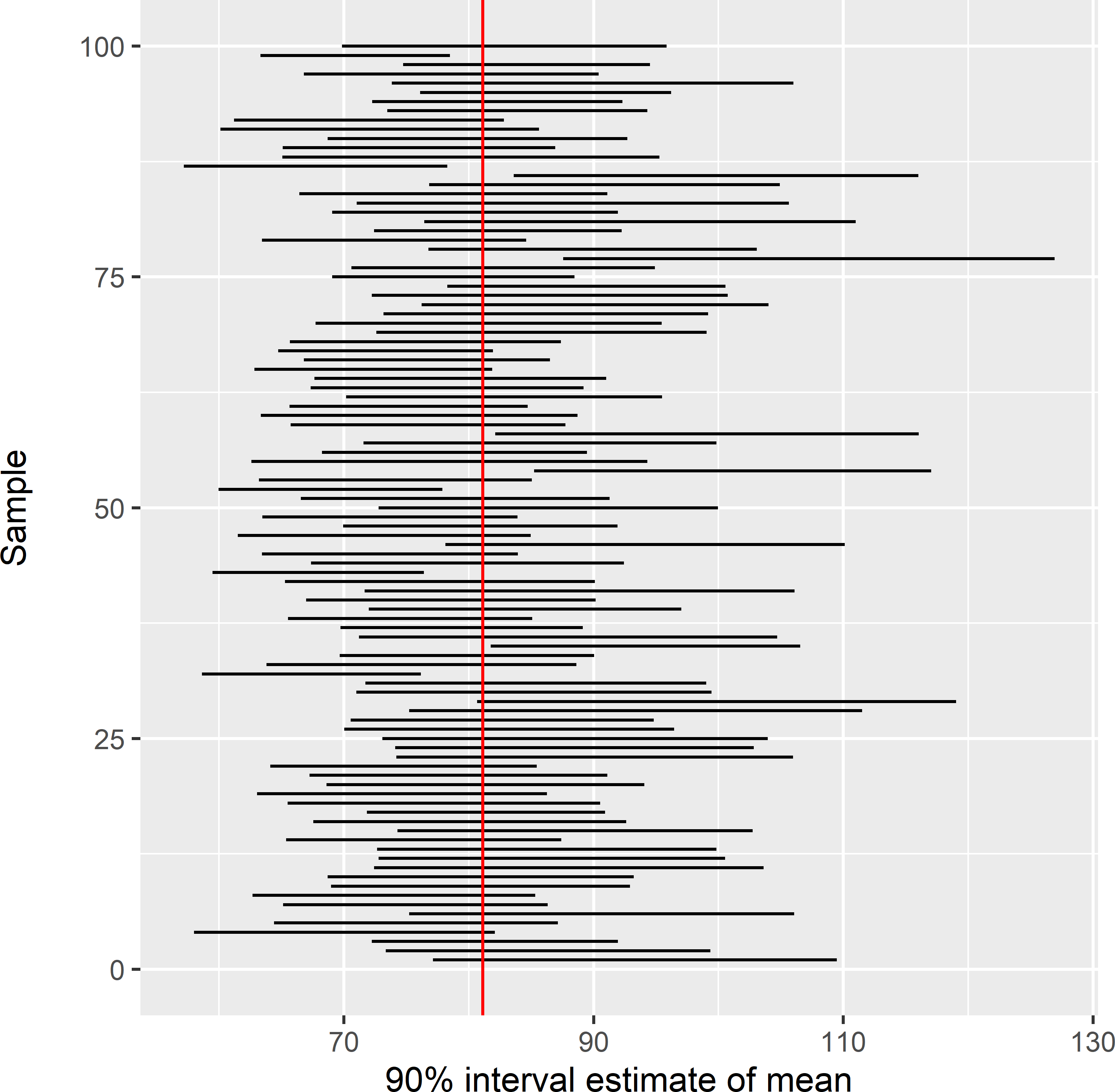
Figure 3.4: Estimated confidence intervals of the mean SOM concentration (g kg^-1) in Voorst, estimated from 100 simple random samples of size 40. The vertical red line is at the true population mean (81.1 g kg^-1).

Out of the 10,000 samples, 1,132 samples do not cover the population mean, i.e., close to the specified 10%. So, a 90% confidence interval is a random interval that contains in the long run the population mean 90% of the time.

3.3.1 Confidence interval for a proportion

Ideally, a confidence interval for a population proportion is based on the binomial distribution of the number of sampling units satisfying a condition (the number of successes). The binomial distribution is a discrete distribution. There are various methods for computing coverage probabilities of confidence intervals for a binomial proportion, see Brown, Cai, and DasGupta (2001) for a discussion. A common method for computing the confidence interval of a proportion is the Clopper-Pearson method. Function BinomCI of package DescTools can be used to compute confidence intervals for proportions (Signorell 2021).

library(DescTools)
n <- 50
k <- 5
print(p.est <- BinomCI(k, n, conf.level = 0.95, method = "clopper-pearson"))

     est     lwr.ci    upr.ci
[1,] 0.1 0.03327509 0.2181354

The confidence interval is not symmetric around the estimated proportion of 0.1. As can be seen below, the upper bound is the proportion at which the probability of 5 or fewer successes is 0.025,

pbinom(q = k, size = n, prob = p.est[3])

[1] 0.025

and the lower bound of the confidence interval is the proportion at which the probability of 5 or more successes is also equal to 0.025. Note that to compute the upper tail probability, we must assign \(k-1 = 4\) to argument q, because with argument lower.tail = FALSE function pbinom computes the probability of \(X>x\), not of \(X \geq x\).

pbinom(q = k - 1, size = n, prob = p.est[2], lower.tail = FALSE)

[1] 0.025

For large sample sizes and for proportions close to 0.5, the confidence interval can be computed with a normal distribution as an approximation to the binomial distribution, using Equation (3.14) for the variance estimator of the estimator of a proportion:

\[\begin{equation} \hat{p} \pm u_{\alpha/2}\sqrt{\frac{\hat{p}(1-\hat{p})}{n-1}} \;. \tag{3.17} \end{equation}\]

This interval is referred to as the Wald interval. It is a fact that unless \(n\) is very large, the actual coverage probability of the Wald interval is poor for \(p\) near 0 or 1. A rule of thumb is that the Wald interval should be used only when \(n \cdot min\{p,(1−p)\}\) is at least 5 or 10. For small \(n\), Brown, Cai, and DasGupta (2001) recommend the Wilson interval and for larger \(n\) the Agresti-Coull interval. These intervals can be computed with function BinomCI of package DescTools.

3.4 Simple random sampling of circular plots

In forest inventory, vegetation surveys, and agricultural surveys, circular sampling plots are quite common. Using circular plots as sampling units is not entirely straightforward, because the study area cannot be partitioned into a finite number of circles that fully cover the study area. The use of circular plots as sampling units can be implemented in two ways (De Vries 1986):

1. sampling from a finite set of fixed circles; and
2. sampling from an infinite set of floating circles.

3.4.1 Sampling from a finite set of fixed circles

Sampling from a finite set of fixed circles is simple, but as we will see this requires an assumption about the distribution of the study variable in the population. In this implementation, the sampling units consist of a finite set of slightly overlapping or non-overlapping fixed circular plots (Figure 3.5). The circles can be constructed as follows. A grid with squares is superimposed on the study area, so that it fully covers the study area. These squares are then substituted by circles with an area equal to the area of the squares, or by non-overlapping tangent circles inscribed in the squares. The radius of the partly overlapping circles equals \(\sqrt{a/\pi}\), with \(a\) the area of the squares, the radius of the non-overlapping circles equals \(\sqrt{a}/2\). In both implementations, the infinite population is replaced by a finite population of circles that does not fully tessellate the study area. When using the partly overlapping circles as sampling units we may avoid overlap by selecting a systematic sample (Chapter 5) of circular plots. The population total can then be estimated by Equation (3.1), substituting \(A/a\) for \(N\), and where \(z_k\) is the total of the \(k\)th circle (sum of observations of all population units in \(k\)th circle). However, no unbiased estimator of the sampling variance of the estimator of the population total or mean is available for this sampling design, see Chapter 5.

With simple random sampling without replacement of non-overlapping circular plots, the finite population total can be estimated by Equation (3.1) and its sampling variance by Equation (3.12). However, the circular plots do not cover the full study area, and as a consequence the total of the infinite population is underestimated. A corrected estimate can be obtained by estimating the mean of the finite population and multiplying this estimated population mean by \(A/a\) (De Vries 1986):

\[\begin{equation} \hat{t}(z)= \frac{A}{a} \hat{\bar{z}}\;, \tag{3.18} \end{equation}\]

with \(\hat{\bar{z}}\) the estimated mean of the finite population. The variance can be estimated by the variance of the estimator of the mean of the finite population, multiplied by the square of \(A/a\). However, we still need to assume that the mean of the finite population is equal to the mean of the infinite population. This assumption can be avoided by sampling from an infinite set of floating circles.

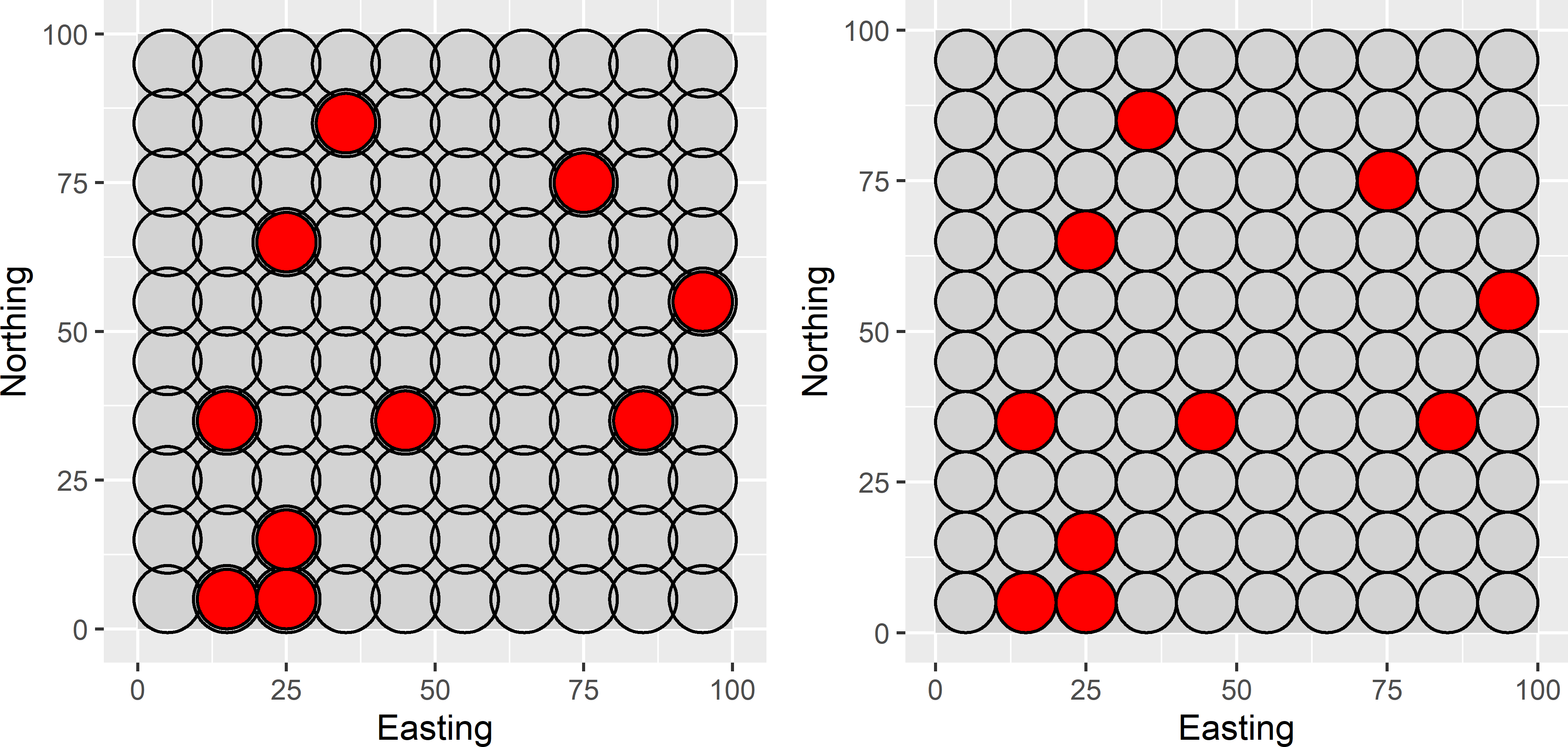
Figure 3.5: Simple random sample of ten circular plots from a square discretised by a finite set of partly overlapping or non-overlapping circular plots.

3.4.2 Sampling from an infinite set of floating circles

A simple random sample of floating circular plots can be selected by simple random sampling of the centres of the plots. The circular plots overlap if two selected points are separated by a distance smaller than the diameter of the circular plots. Besides, when a plot is selected near the border of the study area, a part of the plot is outside the study area. This part is ignored in estimating the population mean or total. To select the centres, the study area must be extended by a zone with a width equal to the radius of the circular plots. This is illustrated in Figure 3.6, showing a square study area of 100 m \(\times\) 100 m. To select ten circular plots with a radius of 5 m from this square, ten points are selected by simple random sampling, using function runif, with -5 as lower limit and 105 as upper limit of the uniform distribution.

set.seed(129)
s1 <- runif(10, min = -5, max = 105)
s2 <- runif(10, min = -5, max = 105)

Two points are selected outside the study area, in the extended zone. For both points, a small part of the circular plot is inside the square. To determine the study variable for these two sampling units, only the part of the plot inside the square is observed. In other words, these two observations have a smaller support than the observations of the other eight plots, see Chapter 1.

In the upper left corner, two sampling units are selected that largely overlap. The intersection of the two circular plots is used twice, to determine the study variable of both sampling units.

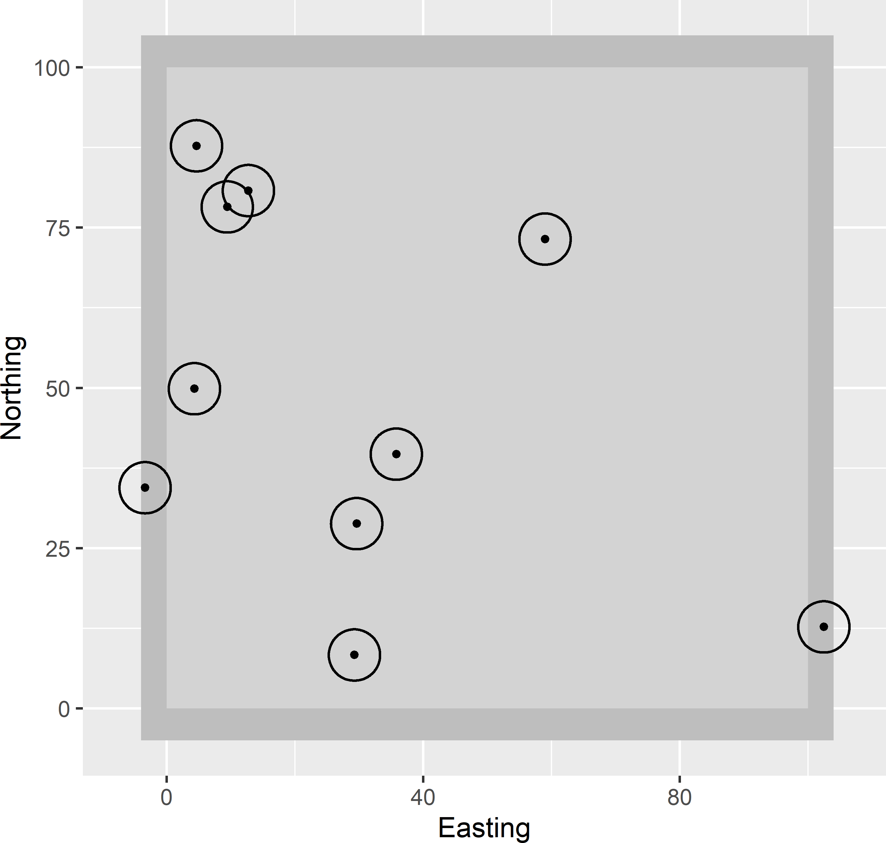
Figure 3.6: Simple random sample of ten floating circular plots from a square.

Given the observations of the selected circular plots, the population total can be estimated by (De Vries 1986)

\[\begin{equation} \hat{t}(z)= \frac{A}{a}\frac{1}{n}\sum_{k \in \mathcal{S}} z_k\;, \tag{3.19} \end{equation}\]

with \(a\) the area of the circle and \(z_k\) the observed total of sampling unit \(k\) (circle). The same estimate of the total is obtained if we divide the observations by \(a\) to obtain a mean per sampling unit:

\[\begin{equation} \hat{t}(z)= A\frac{1}{n}\sum_{k \in \mathcal{S}}\frac{z_k}{a}\;. \tag{3.20} \end{equation}\]

The sampling variance of the estimator of the total can be estimated by

\[\begin{equation} \widehat{V}(\hat{t}(z)) = \left(\frac{A}{a}\right)^2 \frac{\widehat{S^2}(z)}{n}\;, \tag{3.21} \end{equation}\]

with \(\widehat{S^2}(z)\) the estimated population variance of the totals per population unit (circle).

Exercises

8. Write an R script to select a simple random sample of size 40 from Voorst.
   • Use the selected sample to estimate the population mean of the SOM concentration (\(z\) in the data frame) and its standard error.
   • Compute the lower and the upper bound of the 90% confidence interval using the t distribution, and check whether the population mean is covered by the interval.
   • Compare the length of the 90% confidence interval with the length of the 95% interval. Explain the difference in width.
   • Use the selected sample to estimate the total mass of SOM in Mg in the topsoil (\(0-30\) cm) of Voorst. Use as a bulk density 1,500 kg m^-3. The size of the grid cells is 25 m \(\times\) 25 m.
   • Estimate the standard error of the estimated total.
   • Do you think this standard error is a realistic estimate of the uncertainty about the estimated total?

References

Bache, Stefan Milton, and Hadley Wickham. 2020. magrittr: A Forward-Pipe Operator for R. https://CRAN.R-project.org/package=magrittr.

Brown, L. D., T. T. Cai, and A. DasGupta. 2001. “Interval estimation for a binomial proportion - Comment - Rejoinder.” Statistical Science 16 (2): 101–33.

De Vries, P. G. 1986. Sampling Theory for Forest Inventory: A Teach-Yourself Course. New York: Springer-Verlag.

Hutson, Alan D. 1999. “Calculating Nonparametric Confidence Intervals for Quantiles Using Fractional Order Statistics.” Journal of Applied Statistics 26 (3): 343–53. https://doi.org/10.1080/02664769922458.

Hutson, Nicholas, Alan Hutson, and Li Yan. 2019. QuantileNPCI: Nonparametric Confidence Intervals for Quantiles. https://CRAN.R-project.org/package=QuantileNPCI.

Hyndman, R. J., and Y. Fan. 1996. “Sample Quantiles in Statistical Packages.” American Statistician 50 (4): 361–65. https://doi.org/10.2307/2684934.

Lohr, S. L. 1999. Sampling: Design and Analysis. Pacific Grove: Duxbury Press.

———. 2021. survey: Analysis of Complex Survey Samples.

Müller, Kirill, and Hadley Wickham. 2021. Tibble: Simple Data Frames. https://CRAN.R-project.org/package=tibble.

Särndal, C. E., B. Swensson, and J. Wretman. 1992. Model Assisted Survey Sampling. New York: Springer.

Signorell, Andri. 2021. DescTools: Tools for Descriptive Statistics. https://cran.r-project.org/package=DescTools.

---

1. A tibble is a data frame of class tbl_df of package tibble (K. Müller and Wickham 2021). Hereafter, I will use the terms tibble and data frame interchangeably. A traditional data frame is referred to as a data.frame.↩︎