Chapter 13 Model-based optimisation of probability sampling designs
Chapter 10 on model-assisted estimation explained how a linear regression model or a non-linear model obtained with a machine learning algorithm can be used to increase the precision of design-based estimates of the population mean or total using the data collected by a given probability sampling design. This chapter will explain how a model of the study variable can be used at an earlier stage to optimise probability sampling designs. It will show how a model can help in choosing between alternative sampling design types, for instance between systematic random sampling, spreading the sampling units throughout the study area, and two-stage cluster random sampling, resulting in spatial clusters of sampling units. Besides, the chapter will explain how to use a model to optimise the sample size of a given sampling design type, for instance, the number of primary and secondary sampling units with two-stage cluster random sampling. The final section of this chapter is about how a model can be used to optimise spatial strata for stratified simple random sampling.
The models used in this chapter are all geostatistical models of the spatial variation. Chapter 21 is an introduction to geostatistical modelling. Several geostatistical concepts explained in that chapter are needed here to predict the sampling variance.
A general geostatistical model of the spatial variation is
\[\begin{equation} \begin{split} Z(\mathbf{s}) &= \mu(\mathbf{s}) + \epsilon(\mathbf{s}) \\ \epsilon(\mathbf{s}) &\sim \mathcal{N}(0,\sigma^2) \\ \mathrm{Cov}(\epsilon(\mathbf{s}),\epsilon(\mathbf{s}^{\prime})) &= C(\mathbf{h}) \;, \end{split} \tag{13.1} \end{equation}\]
with \(Z(\mathbf{s})\) the study variable at location \(\mathbf{s}\), \(\mu(\mathbf{s})\) the mean at location \(\mathbf{s}\), \(\epsilon(\mathbf{s})\) the residual at location \(\mathbf{s}\), and \(C(\mathbf{h})\) the covariance of the residuals at two locations separated by vector \(\mathbf{h} = \mathbf{s}-\mathbf{s}^{\prime}\). The residuals are assumed to have a normal distribution with zero mean and a constant variance \(\sigma^2\) (\(\mathcal{N}(0,\sigma^2)\)).
The model of the spatial variation has several parameters. In case of a model in which the mean is a linear combination of covariates, these are the regression coefficients associated with the covariates and the parameters of a semivariogram describing the spatial dependence of the residuals. A semivariogram is a model for half the expectation of the squared difference of the study variable or the residuals of a model at two locations, referred to as the semivariance, as a function of the length (and direction) of the vector separating the two locations (Chapter 21).
Using the model to predict the sampling variance of a design-based estimator of a population mean requires prior knowledge of the semivariogram. When data from the study area of interest are available, these data can be used to choose a semivariogram model and to estimate the parameters of the model. If no such data are available, we must make a best guess, based on data collected in other areas. In all cases I recommend keeping the model as simple as possible.
13.1 Model-based optimisation of sampling design type and sample size
Chapter 12 presented methods and formulas for computing the required sample size given various measures to quantify the quality of the survey result. These required sample sizes are for simple random sampling. For other types of sampling design, the required sample size can be approximated by multiplying the required sample size for simple random sampling with the design effect, see Section 12.4. An alternative is to use a model of the spatial variation to predict the sampling variance of the estimator of the mean for the type of sampling design under study and a range of sample sizes, plotting the predicted variance, or standard error, against the sample size, and using this plot inversely to derive the required sample size given a constraint on the sampling variance or standard error.
The computed required sample size applies to several given parameters of the sampling design. For instance, for stratified random sampling, the sample size is computed for a given stratification and sample size allocation scheme, for cluster random sampling for given clusters, and for two-stage cluster random sampling for given primary sampling units (PSUs) and the number of secondary sampling units (SSUs) selected per PSU draw. However, the model can also be used to optimise these sampling design parameters. For stratified random sampling, the optimal allocation can be computed by predicting the population standard deviations within strata and using these predicted standard deviations in Equation (4.17). Even the stratification can be optimised, see Section 13.2. If we have a costs model for two-stage cluster random sampling, the number of PSU draws and the number of SSUs per PSU draw can be optimised.
Model-based prediction of the sampling variance can also be useful to compare alternative types of sampling design at equal total costs or equal variance of the estimated population mean or total. For instance, to compare systematic random sampling, leading to good spatial coverage, and two-stage cluster random sampling, resulting in spatial clusters of observations.
Three approaches for model-based prediction of the sampling variance of a design-based estimator of the population mean, or total, are described: the analytical approach (Subsection 13.1.1), the geostatistical simulation approach (Subsection 13.1.2), and the Bayesian approach (Subsection 13.1.3). In the analytical approach we assume that the mean, \(\mu(\mathbf{s})\) in Equation (13.1), is everywhere the same. This assumption is relaxed in the geostatistical simulation approach. This simulation approach can also accommodate models in which the mean is a linear combination of covariates and/or spatial coordinates to predict the sampling variance. Furthermore, this simulation approach can be used to predict the sampling variance of the estimator of the mean of a trans-Gaussian variable, i.e., a random variable that can be transformed to a Gaussian variable.
The predicted sampling variances of the estimated population mean obtained with the analytical and the geostatistical simulation approach are conditional on the model of the spatial variation. Uncertainty about this model is not accounted for. On the contrary, in the Bayesian approach, we do account for our uncertainty about the assumed model, and we analyse how this uncertainty propagates to the sampling variance of the estimator of the mean.
In some publications, the sampling variance as predicted with a statistical model is referred to as the anticipated variance (Särndal, Swensson, and Wretman (1992), p. 450).
13.1.1 Analytical approach
In the analytical approach, the sampling variance of the estimator of the mean is derived from mean semivariances within the study area and mean semivariances within the sample. Assuming isotropy, the mean semivariances are a function of the separation distance between pairs of points.
The sampling variance of the \(\pi\) estimator of the population mean can be predicted by (Domburg, de Gruijter, and Brus (1994), de Gruijter et al. (2006))
\[\begin{equation} E_{\xi}\{V_p(\hat{\bar{z}})\}=\bar{\gamma}-E_p(\pmb{\lambda}^{\mathrm{T}}\pmb{\Gamma}_{\mathcal{S}}\pmb{\lambda}) \;, \tag{13.2} \end{equation}\]
where \(E_{\xi}(\cdot)\) is the statistical expectation over realisations from the model \(\xi\), \(E_{p}(\cdot)\) is the statistical expectation over repeated sampling with sampling design \(p\), \(V_{p}(\hat{\bar{z}})\) is the variance of the \(\pi\) estimator of the population mean over repeated sampling with sampling design \(p\), \(\bar{\gamma}\) is the mean semivariance of the random variable at two randomly selected locations in the study area, \(\pmb{\lambda}\) is the vector of design-based weights of the units of a sample selected with design \(p\), and \(\pmb{\Gamma}_{\mathcal{S}}\) is the matrix of semivariances between the units of a sample \(\mathcal{S}\) selected with design \(p\).
The mean semivariance \(\bar{\gamma}\) is a model-based prediction of the population variance, or spatial variance, i.e., the model-expectation of the population variance:
\[\begin{equation} \bar{\gamma} = E_{\xi}\{S^2(z)\}\:. \tag{13.3} \end{equation}\]
The mean semivariance \(\bar{\gamma}\) can be calculated by discretising the study area by a fine square grid, computing the matrix with geographical distances between the discretisation nodes, transforming this into a semivariance matrix, and computing the average of all elements of the semivariance matrix. The second term \(E_p(\pmb{\lambda}^{\mathrm{T}}\pmb{\Gamma}_{\mathcal{S}}\pmb{\lambda})\) can be evaluated by Monte Carlo simulation, repeatedly selecting a sample according to design \(p\), calculating \(\pmb{\lambda}^{\mathrm{T}}\pmb{\Gamma}_{\mathcal{S}}\pmb{\lambda}\), and averaging.
This generic procedure is still computationally demanding, but it is the only option for complex spatial sampling designs. For basic sampling designs, the general formula can be worked out. For simple random sampling, the sampling variance can be predicted by
\[\begin{equation} E_{\xi}\{V_\mathrm{SI}(\hat{\bar{z}})\}=\bar{\gamma }/n \;, \tag{13.4} \end{equation}\]
and for stratified simple random sampling by
\[\begin{equation} E_{\xi}\{V_\mathrm{STSI}(\hat{\bar{z}})\}=\sum_{h=1}^H w^2_h \bar{\gamma_h}/n_h \;, \tag{13.5} \end{equation}\]
with \(H\) the number of strata, \(w_h\) the stratum weight (relative size), \(\bar{\gamma}_h\) the mean semivariance of stratum \(h\), and \(n_h\) the number of sampling units of stratum \(h\).
For systematic random sampling, i.e., sampling on a randomly placed grid, the variance can be predicted by
\[\begin{equation} E_{\xi}\{V_\mathrm{SY}(\hat{\bar{z}})\}=\bar{\gamma} - E_{\mathrm{SY}}(\bar{\gamma}_{\mathrm{SY}}) \;, \tag{13.6} \end{equation}\]
with \(E_{\mathrm{SY}}(\bar{\gamma}_{\mathrm{SY}})\) the design-expectation, i.e., the expectation over repeated systematic sampling, of the mean semivariance within the grid. With systematic random sampling, the number of grid points within the study area can vary among samples, as well as the spatial pattern of the points (Chapter 5). Therefore, multiple systematic random samples must be selected, and the average of the mean semivariance within the systematic sample must be computed.
The analytical approach is illustrated with the data of agricultural field Leest (Hofman and Brus 2021). Nitrate-N (NO\(_3\)-N) in kg ha-1 in the layer \(0-90\) cm, using a standard soil density of 1,500 kg m-3, is measured at 30 points. In the next code chunk, these data are used to compute a sample semivariogram using the method-of-moments with function variogram, see Chapter 21. A spherical model without nugget is fitted to the sample semivariogram using function fit.variogram. The numbers in this plot are the numbers of pairs of points used to compute the semivariances.
library(gstat)
coordinates(sampleLeest) <- ~ s1 + s2
vg <- variogram(N ~ 1, data = sampleLeest)
vgm_MoM <- fit.variogram(
  vg, model = vgm(model = "Sph", psill = 2000, range = 20))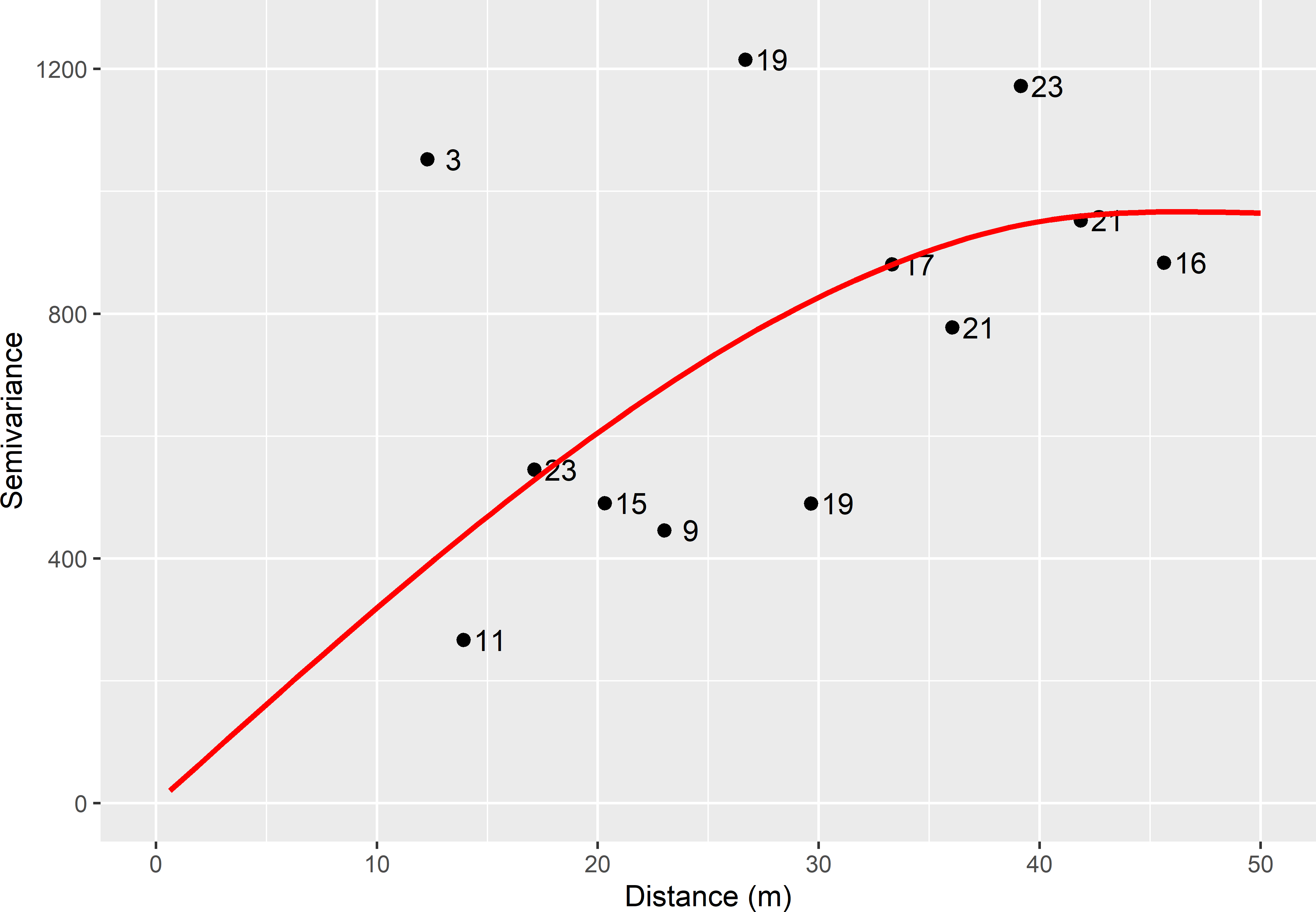
Figure 13.1: Sample semivariogram and fitted spherical model for NO3-N in field Leest. The numbers refer to point-pairs used in computing semivariances.
The few data lead to a very noisy sample semivariogram. For the moment, I ignore my uncertainty about the semivariogram parameters; Subsection 13.1.3 will show how we can account for our uncertainty about the semivariogram parameters in model-based prediction of the sampling variance. A spherical semivariogram model without nugget is fitted to the sample semivariogram, i.e., the intercept is 0. The fitted range of the model is 45 m, and the fitted sill equals 966 (kg ha-1)2. The fitted semivariogram is used to predict the sampling variance for three sampling designs: simple random sampling, stratified simple random sampling, and systematic random sampling. The costs for these three design types will be about equal, as the study area is small, so that the access time of the sampling points selected with the three designs is about equal. The sample size of the evaluated sampling designs is 25 points. As for systematic random sampling, the number of points varies among the samples, this sampling design has an expected sample size of 25 points.
Simple random sampling
For simple random sampling, we must compute the mean semivariance within the field (Equation (13.4)). As shown in the next code chunk, the mean semivariance is approximated by discretising the field by a square grid of 2,000 points, computing the 2,000 \(\times\) 2,000 matrix with distances between all pairs of discretisation nodes, transforming this distance matrix into a semivariance matrix using function variogramLine of package gstat (E. J. Pebesma 2004), and finally averaging the semivariances. Note that in this case we do not need to replace the zeroes on the diagonal of the semivariance matrix by the nugget, as a model without nugget is fitted. The geopackage file is read with function read_sf of package sf (E. Pebesma 2018), resulting in a simple feature object. The projection attributes of this object are removed with function st_set_crs. The centres of square grid cells are selected with function st_make_grid. The centres inside the field are selected with mygrid[field], and finally the coordinates are extracted with function st_coordinates.
field <- read_sf(system.file("extdata/leest.gpkg", package = "sswr")) %>%
  st_set_crs(NA_crs_)
mygrid <- st_make_grid(field, cellsize = 2, what = "centers")
mygrid <- mygrid[field] %>%
  st_coordinates(mygrid)
H <- as.matrix(dist(mygrid))
G <- variogramLine(vgm_MoM, dist_vector = H)
m_semivar_field <- mean(G)
n <- 25
Exi_V_SI <- m_semivar_field / n
The model-based prediction of the sampling variance of the estimator of the mean with this design equals 35.0.
Stratified simple random sampling
The strata of the stratified simple random sampling design are compact geographical strata of equal size (Section 4.6). The number of geostrata is equal to the sample size, 25 points, so that we have one point per stratum. With this design, the sampling points are reasonably well spread over the field, but not as good as with systematic random sampling. To predict the sampling variance, we must compute the mean semivariances within the geostrata, see Equation (13.5). Note that the stratum weights are constant as the strata have equal size, \(w_h = 1/n\), and that \(n_h=1\). Therefore, Equation (13.5) reduces to
\[\begin{equation} E_{\xi}\{V_\mathrm{STSI}(\hat{\bar{z}})\}=\frac{1}{n^2}\sum_{h=1}^H \bar{\gamma_h} \;. \tag{13.7} \end{equation}\]
The next code chunk shows the computation of the mean semivariance per stratum and the model-based prediction of the sampling variance of the estimator of the mean. The matrix with the coordinates is first converted to a tibble with function as_tibble.
library(spcosa)
mygrid <- mygrid %>%
  as_tibble() %>%
  setNames(c("x1", "x2"))
gridded(mygrid) <- ~ x1 + x2
mygeostrata <- stratify(mygrid, nStrata = n, equalArea = TRUE, nTry = 10) %>%
  as("data.frame")
m_semivar_geostrata <- numeric(length = n)
for (i in 1:n) {
 ids <- which(mygeostrata$stratumId == (i - 1))
 mysubgrd <- mygeostrata[ids, ]
 H_geostratum <- as.matrix(dist(mysubgrd[, c(2, 3)]))
 G_geostratum <- variogramLine(vgm_MoM, dist_vector = H_geostratum)
 m_semivar_geostrata[i] <- mean(G_geostratum)
}
Exi_V_STSI <- sum(m_semivar_geostrata) / n^2
The model-based prediction of the sampling variance with this design equals 13.5 (kg ha-1)2, which is much smaller than with simple random sampling. The large stratification effect can be explained by the assumed strong spatial structure of NO\(_3\)-N in the agricultural field and the improved geographical spreading of the sampling points, see Figure 13.1.
Systematic random sampling
To predict the sampling variance for systematic random sampling with an expected sample size of 25 points, we must compute the design-expectation of the mean semivariance within the systematic sample (Equation (13.6)). As shown in the next code chunk, I approximated this expectation by selecting 100 systematic random samples, computing the mean semivariance for each sample, and averaging. Finally, the model-based prediction of the sampling variance is computed by subtracting the average of the mean semivariances within a systematic sample from the mean semivariance within the field computed above.
set.seed(314)
m_semivar_SY <- numeric(length = 100)
for (i in 1:100) {
  mySYsample <- spsample(x = mygrid, n = n, type = "regular") %>%
    as("data.frame")
  H_SY <- as.matrix(dist(mySYsample))
  G_SY <- variogramLine(vgm_MoM, dist_vector = H_SY)
  m_semivar_SY[i] <- mean(G_SY)
}
Exi_V_SY <- m_semivar_field - mean(m_semivar_SY)
The model-based prediction of the sampling variance of the estimator of the mean with this design equals 8.3 (kg ha-1)2, which is smaller than that of stratified simple random sampling. This can be explained by the improved geographical spreading of the sampling points with systematic random sampling as compared to stratified simple random sampling with compact geographical strata.
13.1.1.1 Bulking soil aliquots into a composite sample
If the soil aliquots collected at the points of the stratified random sample are bulked into a composite, as is usually done in soil testing of agricultural fields, the procedure for predicting the variance of the estimator of the mean is slightly different. Only the composite sample is analysed in a laboratory on NO\(_3\)-N, not the individual soil aliquots. This implies that the contribution of the measurement error to the total uncertainty about the population mean is larger. To predict the sampling variance in this situation, we need the semivariogram of errorless measurements of NO\(_3\)-N, i.e., of the true NO\(_3\)-N contents of soil aliquots collected at points. The sill of this semivariogram will be smaller than the sill of the semivariogram of measured NO\(_3\)-N data. A simple option is to subtract an estimate of the measurement error variance from the semivariogram of measured NO\(_3\)-N data that contain a measurement error. So, the measurement error variance is subtracted from the nugget. This may lead to negative nuggets, which is not allowed (a variance cannot be negative). The preferable alternative is to add the measurement error variance to the diagonal of the covariance matrix of the data in fitting the model with maximum likelihood, see function ll in Subsection 13.1.3.
Exercises
- Write an R script to predict the sampling variance of the estimator of the mean of NO\(_3\)-N of agricultural field Leest, for simple random sampling and a sample size of 25 points. Use in prediction a spherical semivariogram with a nugget of 483, a partial sill of 483, and a range of 44.6 m. The sum of the nugget and partial sill (966) is equal to the sill of the semivariogram used above in predicting sampling variances. Compare the predicted sampling variance with the predicted sampling variance for the same sampling design, obtained with the semivariogram without nugget. Explain the difference.
- Write an R script to compute the required sample size for simple random sampling of agricultural field Leest, for a maximum length of a 95% confidence interval of 20. Use the semivariogram without nugget in predicting the sampling variance. See Section 12.2 (Equation (12.7)) for how to compute the required sample size given a prior estimate of the standard deviation of the study variable in the population.
- Do the same for systematic random sampling. Note that for this sampling design, no such formula is available. Predict for a series of expected sample sizes, \(n = 5,6,\dots , 40\), the sampling variance of the estimator of the mean, using Equation (13.6). Approximate \(E_{\mathrm{SY}}(\bar{\gamma}_{\mathrm{SY}})\) from ten repeated selections. Compute the length of the confidence interval from the predicted sampling variances, and plot the interval length against the sample size. Finally, determine the required sample size for a maximum length of 20. What is the design effect for an expected sample size of 34 points (the required sample size for simple random sampling)? See Equation (12.13). Also compute the design effect for expected sample sizes of \(5,6,\dots , 40\). Explain why the design effect is not constant.
13.1.2 Geostatistical simulation approach
The alternative to the analytical approach is to use a geostatistical simulation approach. It is computationally more demanding, but an advantage of this approach is its flexibility. It can also be used to predict the sampling variance of the estimator of the mean using a geostatistical model with a non-constant mean. And besides, this approach can also handle trans-Gaussian variables, i.e., variables whose distribution can be transformed into a normal distribution. In Subsection 13.1.3, geostatistical simulation is used to predict the variance of the estimator of the mean of a lognormal variable.
The geostatistical simulation approach for predicting the sampling variance of a design-based estimator of the population mean involves the following steps:
- Select a large number \(S\) of random samples with sampling design \(p\).
- Use the model to simulate values of the study variable for all sampling points.
- Estimate for each sample the population mean, using the design-based estimator of the population mean for sampling design \(p\). This results in \(S\) estimated population means.
- Compute the variance of the \(S\) estimated means.
- Repeat steps 1 to 4 \(R\) times, and compute the mean of the \(R\) variances.
This approach is illustrated with the western part of the Amhara region in Ethiopia (hereafter referred to as West-Amhara) where a large sample is available with organic matter data in the topsoil (SOM) in decagram per kg dry soil (dag kg-1; 1 decagram = 10 gram). The soil samples are collected along roads (see Figure 17.5). It is a convenience sample, not a probability sample, so these sample data cannot be used in design-based or model-assisted estimation of the mean or total soil carbon stock in the study area. However, the data can be used to model the spatial variation of the SOM concentration, and this geostatistical model can then be used to design a probability sample for design-based estimation of the total mass of SOM. Apart from the point data of the SOM concentration, maps of covariates are available, such as a digital elevation model and remote sensing reflectance data. In the next code chunk, four covariates are selected to model the mean of the SOM concentration: elevation (dem), average near infrared reflectance (rfl-NIR), average red reflectance (rfl-red), and average land surface temperature (lst). I assume a normal distribution for the residuals of the linear model. The model parameters are estimated by restricted maximum likelihood (REML), using package geoR (Ribeiro Jr et al. 2020), see Subsection 21.5.2 for details on REML estimation of a geostatistical model. As a first step, the projected coordinates of the sampling points are changed from m into km using function mutate. Using coordinates in m in function likfit could not find an optimal estimate for the range.
library(geoR)
sampleAmhara <- sampleAmhara %>%
  mutate(s1 = s1 / 1000, s2 = s2 / 1000)
dGeoR <- as.geodata(obj = sampleAmhara, header = TRUE,
  coords.col = c("s1", "s2"), data.col = "SOM",
  covar.col = c("dem", "rfl_NIR", "rfl_red", "lst"))
vgm_REML <- likfit(geodata = dGeoR,
  trend = ~ dem + rfl_NIR + rfl_red + lst,
  cov.model = "spherical", ini.cov.pars = c(1, 50), nugget = 0.2,
  lik.method = "REML", messages = FALSE)
The estimated parameters of the residual semivariogram of the SOM concentration are shown in Table 22.2. The estimated regression coefficients are 12.9 for the intercept, 0.922 for elevation (dem), 7.41 for NIR reflectance, -10.42 for red reflectance, and -0.039 for land surface temperature.
Package gstat is used for geostatistical simulation, and therefore first the REML estimates of the semivariogram parameters are passed to function vgm using arguments nugget, psill, and range of function vgm of this package.
vgm_REML_gstat <- vgm(model = "Sph", nugget = vgm_REML$tausq,
  psill = vgm_REML$sigmasq, range = vgm_REML$phi)
The fitted model of the spatial variation of the SOM concentration is used to compare systematic random sampling and two-stage cluster random sampling at equal variances of the estimator of the mean.
Systematic random sampling
One hundred systematic random samples (\(S=100\)) with an expected sample size of 50 points (\(E[n]=50\)) are selected. The four covariates at the selected sampling points are extracted by overlaying the SpatialPointsDataFrame mySYsamples and the SpatialPixelsDataFrame grdAmhara with function over of package sp (E. J. Pebesma and Bivand 2005). Values at the sampling points are simulated by sequential Gaussian simulation (Goovaerts 1997), using function krige with argument nsim = 1 of package gstat. Argument dummy is set to TRUE to enforce unconditional simulation.
Note that by first drawing 100 samples, followed by simulating values of \(z\) at the selected sampling points, instead of first simulating values of \(z\) at the nodes of a discretisation grid, followed by selecting samples and overlaying with the simulated field, the simulated values of points in the same discretisation cell differ, so that we account for the infinite number of points in the population.
With systematic random sampling, the sample mean is an approximately unbiased estimator of the population mean (Chapter 5). Therefore, of each sample the mean of the simulated values is computed, using function tapply. Finally, the variance of the 100 sample means is computed. This is a conditional variance, conditional on the simulated values. In the code chunk below, the whole procedure is repeated 100 times (\(R=100\)), leading to 100 conditional variances of sample means.
grdAmhara <- grdAmhara %>%
  mutate(s1 = s1 / 1000, s2 = s2 / 1000)
gridded(grdAmhara) <- ~ s1 + s2
S <- R <- 100
v_mzsim_SY <- numeric(length = R)
set.seed(314)
for (i in 1:R) {
  mySYsamples <- NULL
  for (j in 1:S) {
    xy <- spsample(x = grdAmhara, n = 50, type = "regular")
    mySY <- data.frame(
      s1 = xy$x1, s2 = xy$x2, sample = rep(j, length(xy)))
    mySYsamples <- rbind(mySYsamples, mySY)
  }
  coordinates(mySYsamples) <- ~ s1 + s2
  res <- over(mySYsamples, grdAmhara)
  mySYs <- data.frame(mySYsamples, res[, c("dem", "rfl_NIR", "rfl_red", "lst")])
  coordinates(mySYs) <- ~ s1 + s2
  zsim <- krige(
    dummy ~ dem + rfl_NIR + rfl_red + lst,
    locations = mySYs, newdata = mySYs,
    model = vgm_REML_gstat, beta = vgm_REML$beta,
    nmax = 20, nsim = 1,
    dummy = TRUE,
    debug.level = 0) %>% as("data.frame")
  m_zsim <- tapply(zsim$sim1, INDEX = mySYs$sample, FUN = mean)
  v_mzsim_SY[i] <- var(m_zsim)
}
grdAmhara <- as_tibble(grdAmhara)The mean of the 100 conditional variances equals 0.015 (dag kg-1)2. This is a Monte Carlo approximation of the model-based prediction of the sampling variance of the ratio estimator of the mean for systematic random sampling with an expected sample size of 50.
Two-stage cluster random sampling
Due to the geographical spreading of the sampling points with systematic random sampling, the accuracy of the estimated mean is expected to be high compared to that of other sampling designs of the same size. However, with large areas, the time needed for travelling to the sampling points can become substantial, lowering the sampling efficiency. With large areas, sampling designs leading to spatial clusters of sampling points can be an attractive alternative. One option then is two-stage cluster random sampling, see Chapter 7. The question is whether this alternative design is more efficient than systematic random sampling.
In the next code chunk, 100 compact geostrata (see Section 4.6) are computed for West-Amhara. Here, these geostrata are not used as strata in stratified random sampling, but as PSUs in two-stage cluster random sampling. The difference is that in stratified random sampling from each geostratum at least one sampling unit is selected, whereas in two-stage cluster random sampling only a randomly selected subset of the geostrata is sampled. The compact geostrata, used as PSUs, are computed with function kmeans, and as a consequence the PSUs do not have equal size, see output of code chunk below. This is not needed in two-stage cluster random sampling, see Chapter 7. If PSUs of equal size are preferred, then these can be computed with function stratify of package spcosa with argument equalArea = TRUE, see Section 4.6.
set.seed(314)
res <- kmeans(
  grdAmhara[, c("s1", "s2")], iter.max = 1000, centers = 100, nstart = 100)
mypsus <- res$cluster
psusize <- as.numeric(table(mypsus))
summary(psusize)
Min. 1st Qu. Median Mean 3rd Qu. Max.
79.0 103.8 109.0 108.4 113.0 131.0 In the next code chunks, I assume that the PSUs are selected with probabilities proportional to their size and with replacement (ppswr sampling), see Chapter 7. In Section 7.1 formulas are presented for computing the optimal number of PSU draws and SSU draws per PSU draw. The optimal sample sizes are a function of the pooled variance of PSU means, \(S^2_{\mathrm{b}}\), and the pooled variance of secondary units (points) within the PSUs, \(S^2_{\mathrm{w}}\). In the current subsection, these variance components are predicted with the geostatistical model.
As a first step, a large number of maps are simulated.
grdAmhara$psu <- mypsus
coordinates(grdAmhara) <- ~ s1 + s2
set.seed(314)
zsim <- krige(
  dummy ~ dem + rfl_NIR + rfl_red + lst,
  locations = grdAmhara, newdata = grdAmhara,
  model = vgm_REML_gstat, beta = vgm_REML$beta,
  nmax = 20, nsim = 1000,
  dummy = TRUE, debug.level = 0) %>% as("data.frame")
zsim <- zsim[, -c(1, 2)]
For each simulated field, the means of the PSUs and the variances of the simulated values within the PSUs are computed using function tapply in function apply.
m_zsim_psu <- apply(zsim, MARGIN = 2, FUN = function(x)
  tapply(x, INDEX = grdAmhara$psu, FUN = mean))
v_zsim_psu <- apply(zsim, MARGIN = 2, FUN = function(x)
  tapply(x, INDEX = grdAmhara$psu, FUN = var))
Next, for each simulated field, the pooled variance of PSU means and the pooled variance within PSUs are computed, and finally these pooled variances are averaged over all simulated fields. The averages are approximations of the model-expectations of the pooled between unit and within unit variances, \(E_{\xi}[S^2_{\mathrm{b}}]\) and \(E_{\xi}[S^2_{\mathrm{w}}]\).
p_psu <- psusize / sum(psusize)
S2b <- apply(m_zsim_psu, MARGIN = 2, FUN = function(x)
  sum(p_psu * (x - sum(p_psu * x))^2))
S2w <- apply(v_zsim_psu, MARGIN = 2, FUN = function(x)
  sum(p_psu * x))
Exi_S2b <- mean(S2b)
Exi_S2w <- mean(S2w)
The optimal sample sizes are computed for a simple linear costs model: \(C = c_0 + c_1n + c_2nm\), with \(c_0\) the fixed costs, \(c_1\) the access costs per PSU, including the access costs of the SSUs (points) within a given PSU, and \(c_2\) the observation costs per SSU. In the next code chunk, I use \(c_1=2\) and \(c_2=1\). For the optimal sample sizes only the ratio of \(c_1\) and \(c_2\) is important, not their absolute values.
Given values for \(c_1\) and \(c_2\), the optimal number of PSU draws \(n\) and the optimal number of SSU draws per PSU draw \(m\) are computed, required for a sampling variance of the estimator of the mean equal to the sampling variance with systematic random sampling of 50 points, see Equations (7.9) and (7.10).
c1 <- 2; c2 <- 1
nopt <- 1 / Exi_vmz_SY * (sqrt(Exi_S2w * Exi_S2b) * sqrt(c2 / c1) + Exi_S2b)
mopt <- sqrt(Exi_S2w / Exi_S2b) * sqrt(c1 / c2)
The optimal number of PSU draws is 26, and the optimal number of points per PSU draw equals 5. The total number of sampling points is 26 \(\times\) 5 = 130. This is much larger than the sample size of 50 obtained with systematic random sampling. The total observation costs therefore are substantially larger. However, the access time can be substantially smaller due to the spatial clustering of sampling points. To answer the question of whether the costs saved by this reduced access time outweigh the extra costs of observation, the model for the access costs and observation costs must be further developed.
13.1.3 Bayesian approach
The model-based prediction of the variance of the design-based estimator of the population mean for a given sampling design is conditional on the model. If we change the model type or the model parameters, the predicted sampling variance also changes. In most situations we are quite uncertain about the model, even in situations where we have data that can be used to estimate the model parameters, as in the West-Amhara case study. Instead of using the best estimated model to predict the sampling variance as done in the previous sections, we may prefer to account for the uncertainty about the model parameters. This can be done through a Bayesian approach, in which the legacy data are used to update a prior distribution of the model parameters to a posterior distribution. For details about a Bayesian approach for estimating model parameters, see Section 22.5. A sample from the posterior distribution of the model parameters is used one-by-one to predict the sampling variance. This can be done either analytically, as described in Subsection 13.1.1, or through geostatistical simulation, as described in Subsection 13.1.2. Both approaches result in a distribution of sampling variances, reflecting our uncertainty about the sampling variance of the estimator of the population mean due to uncertainty about the model parameters. The mean or median of the distribution of sampling variances can be used as the predicted sampling variance.
The Bayesian approach is illustrated with a case study on predicting the sampling variance of NO\(_3\)-N in agricultural field Melle in Belgium (Hofman and Brus 2021). As for field Leest used in Subsection 13.1.1, data of NO\(_3\)-N are available at 30 points. The sampling points are approximately on the nodes of a square grid with a spacing of about 4.5 m. As a first step, I check whether we can safely assume that the data come from a normal distribution.
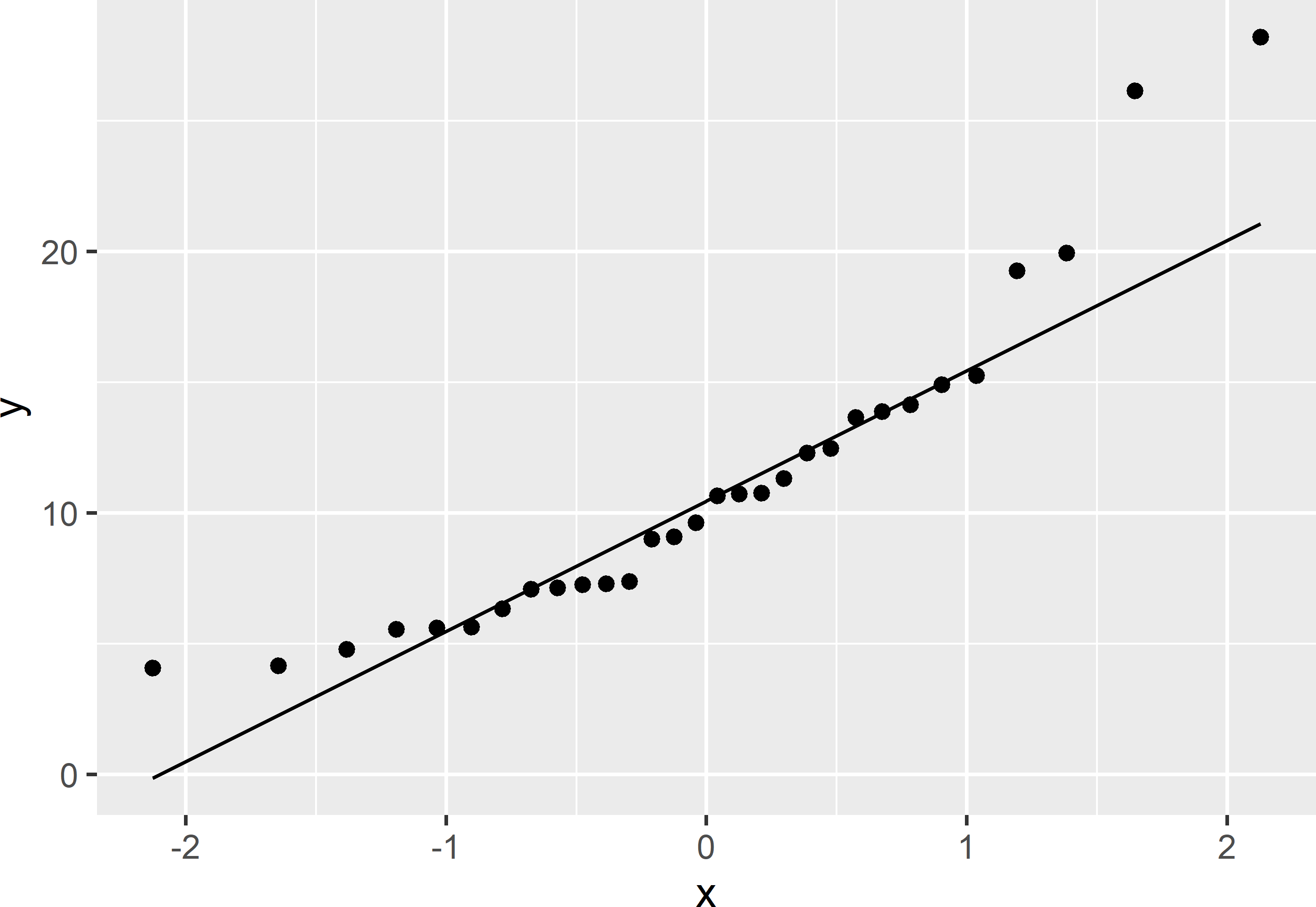
Figure 13.2: Q-Q plot of NO3-N of field Melle.
The Q-Q plot (Figure 13.2) shows that a normal distribution is not very likely: there are too many large values, i.e., the distribution is skewed to the right. Also the p-value of the Shapiro-Wilk test shows that we should reject the null hypothesis of a normal distribution for the data: \(p=0.0028\). I therefore proceed with the natural log of NO\(_3\)-N, in short lnN.
As a first step, the semivariogram of lnN is estimated by maximum likelihood (Subsection 21.4.2). An exponential semivariogram model is assumed, see Equation (21.13).
The likelihood function is defined, using a somewhat unusual parameterisation, tailored to the Markov chain Monte Carlo (MCMC) sampling from the posterior distribution of the semivariogram parameters. In MCMC a Markov chain of sampling units (vectors with semivariogram parameters) is generated using the previous sampling unit to randomly generate the next sampling unit (Gelman et al. (2013), chapter 11). In MCMC sampling, the probability of accepting a proposed sampling unit \(\pmb{\theta}^*\) is a function of the ratio of the posterior density of the proposed sampling unit and that of the current sampling unit, \(f(\pmb{\theta}^*|\mathbf{z})/f(\pmb{\theta}_{t-1}|\mathbf{z})\), so that the normalising constant, the denominator of Equation (12.15), cancels.
library(mvtnorm)
ll <- function(thetas) {
  sill <- 1 / thetas[1]
  psill <- thetas[2] * sill
  nugget <- sill - psill
  vgmodel <- vgm(
    model = model, psill = psill, range = thetas[3], nugget = nugget)
  C <- variogramLine(vgmodel, dist_vector = D, covariance = TRUE)
  XCX <- crossprod(X, solve(C, X))
  XCz <- crossprod(X, solve(C, z))
  betaGLS <- solve(XCX, XCz)
  mu <- as.numeric(X %*% betaGLS)
  logLik <- dmvnorm(x = z, mean = mu, sigma = C, log = TRUE)
  logLik
}
Next, initial estimates of the semivariogram parameters are computed by maximising the likelihood, using function optim.
lambda.ini <- 1 / var(sampleMelle$lnN)
xi.ini <- 0.5
phi.ini <- 20
pars <- c(lambda.ini, xi.ini, phi.ini)
D <- as.matrix(dist(sampleMelle[, c("s1", "s2")]))
X <- matrix(1, nrow(sampleMelle), 1)
z <- sampleMelle$lnN
model <- "Exp"
vgML <- optim(pars, ll, control = list(fnscale = -1),
  lower = c(1e-6, 0, 1e-6), upper = c(1000, 1, 150), method = "L-BFGS-B")
The maximum likelihood (ML) estimates of the semivariogram parameters are used as initial values in MCMC sampling. A uniform prior is used for the inverse of the sill parameter, \(\lambda=1/\sigma^2\), with a lower bound of \(10^{-6}\) and an upper bound of 1. For the relative nugget, \(\tau^2/\sigma^2\), a uniform prior is assumed with a lower bound of 0 and an upper bound of 1. For the distance parameter \(\phi\) of the exponential semivariogram a uniform prior is assumed, with a lower bound of \(10^{-6}\) m and an upper bound of 150 m.
These priors can be defined by function createUniformPrior of package BayesianTools (Hartig, Minunno, and Paul 2019). Function createBayesianSetup is then used to define the setup of the MCMC sampling, specifying the likelihood function, the prior, and the vector with best prior estimates of the model parameters, passed to function createBayesianSetup using argument best. Argument sampler of function runMCMC specifies the type of MCMC sampler. I used the differential evolution algorithm of ter Braak and Vrugt (2008). Argument start of function getSample specifies the burn-in period, i.e., the number of first samples that are discarded to diminish the influence of the initial semivariogram parameter values. Argument numSamples specifies the sample size, i.e., the number of saved vectors with semivariogram parameter values, drawn from the posterior distribution.
library(BayesianTools)
priors <- createUniformPrior(lower = c(1e-6, 0, 1e-6),
                             upper = c(1000, 1, 150))
bestML <- c(vgML$par[1], vgML$par[2], vgML$par[3])
setup <- createBayesianSetup(likelihood = ll, prior = priors,
  best = bestML, names = c("lambda", "xi", "phi"))
set.seed(314)
res <- runMCMC(setup, sampler = "DEzs")
MCMCsample <- getSample(res, start = 1000, numSamples = 1000) %>% data.frame()
Figure 13.3 shows several semivariograms, sampled by MCMC from the posterior distribution of the estimated semivariogram parameters.
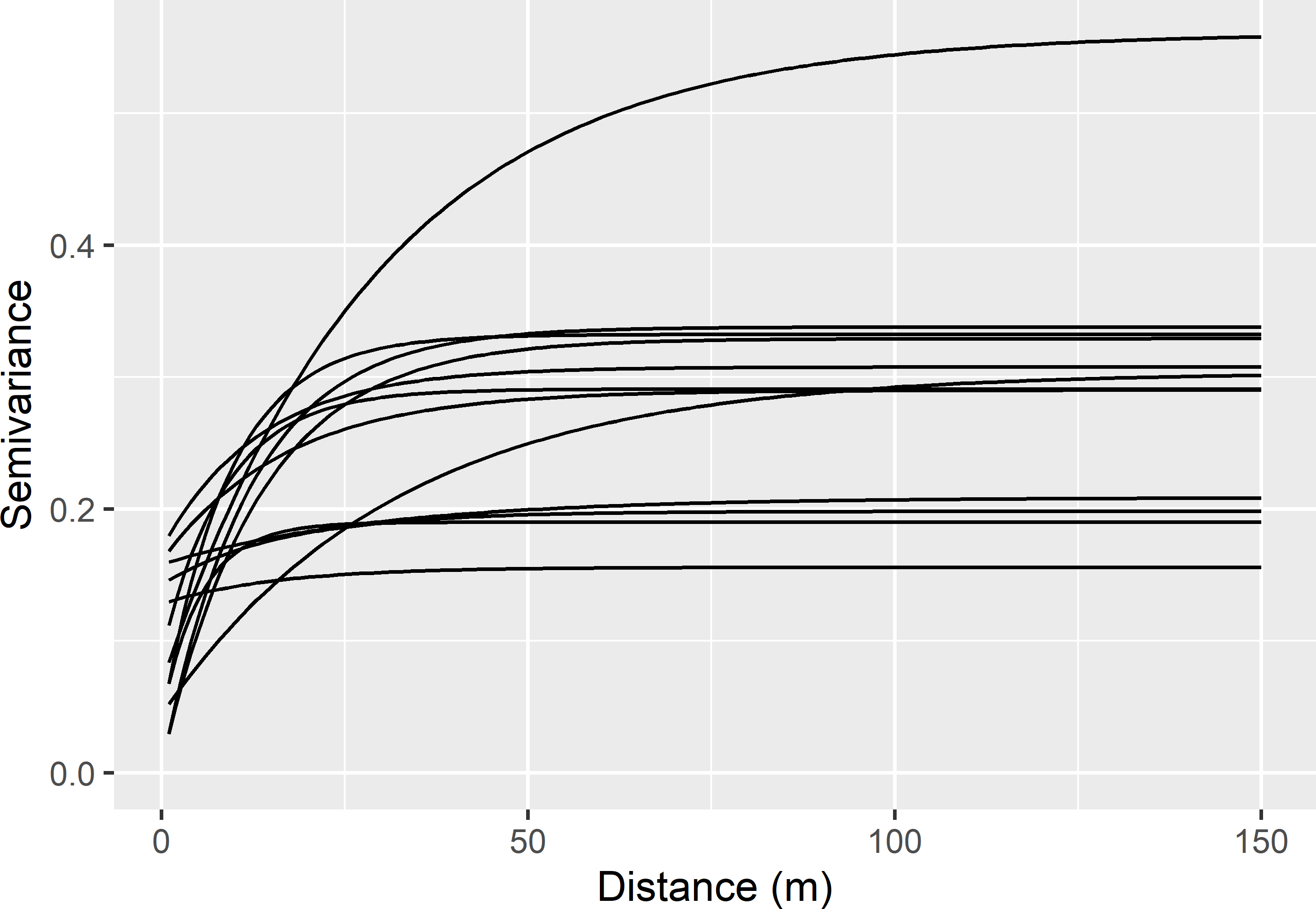
Figure 13.3: Semivariograms of the natural log of NO3-N for field Melle obtained by MCMC sampling from posterior distribution of the estimated semivariogram parameters.
The evaluated sampling design is the same as used in Subsection 13.1.1 for field Leest: stratified simple random sampling, using compact geographical strata of equal size, a total sample size of 25 points, and one point per stratum.
The next step is to simulate with each of the sampled semivariograms a large number of maps of lnN. This is done by sequential Gaussian simulation, conditional on the available data. The simulated values are backtransformed. Each simulated map is then used to compute the variance of the simulated values within the geostrata \(S^2_h\). These stratum variances are used to compute the sampling variance of the estimator of the mean. Plugging \(w_h = 1/n\) (all strata have equal size) into Equation (4.4) and using \(n_h=1\) in Equation (4.5) yield (compare with Equation (13.7))
\[\begin{equation} V(\hat{\bar{z}}) = \frac{1}{n^2}\sum_{h=1}^H S^2_h \;. \tag{13.8} \end{equation}\]
In the code chunk below, I use the first 100 sampled semivariograms to simulate with each semivariogram 100 maps.
V <- matrix(data = NA, nrow = 100, ncol = 100)
coordinates(sampleMelle) <- ~ s1 + s2
set.seed(314)
for (i in 1:100) {
  sill <- 1 / MCMCsample$lambda[i]
  psill <- MCMCsample$xi[i] * sill
  nug <- sill - psill
  range <- MCMCsample$phi[i]
  vgmdl <- vgm(model = "Exp", nugget = nug, psill = psill, range = range)
  ysim <- krige(
    lnN ~ 1, locations = sampleMelle, newdata = mygrid,
    model = vgmdl,
    nmax = 20, nsim = 100,
    debug.level = 0) %>% as("data.frame")
  zsim <- exp(ysim[, -c(1, 2)])
  S2h <- apply(zsim, MARGIN = 2, FUN = function(x)
    tapply(x, INDEX = as.factor(mygeostrata$stratumId), FUN = var))
  V[i, ] <- 1 / n^2 * apply(S2h, MARGIN = 2, FUN = sum)
}
Figure 13.4 shows 16 maps simulated with the first four semivariograms. The four maps in a row (a to d) are simulated with the same semivariogram. All maps show that the simulated data have positive skew, which is in agreement with the prior data. The data obtained by simulating from a lognormal distribution are always strictly positive. This is not guaranteed when simulating from a normal distribution.
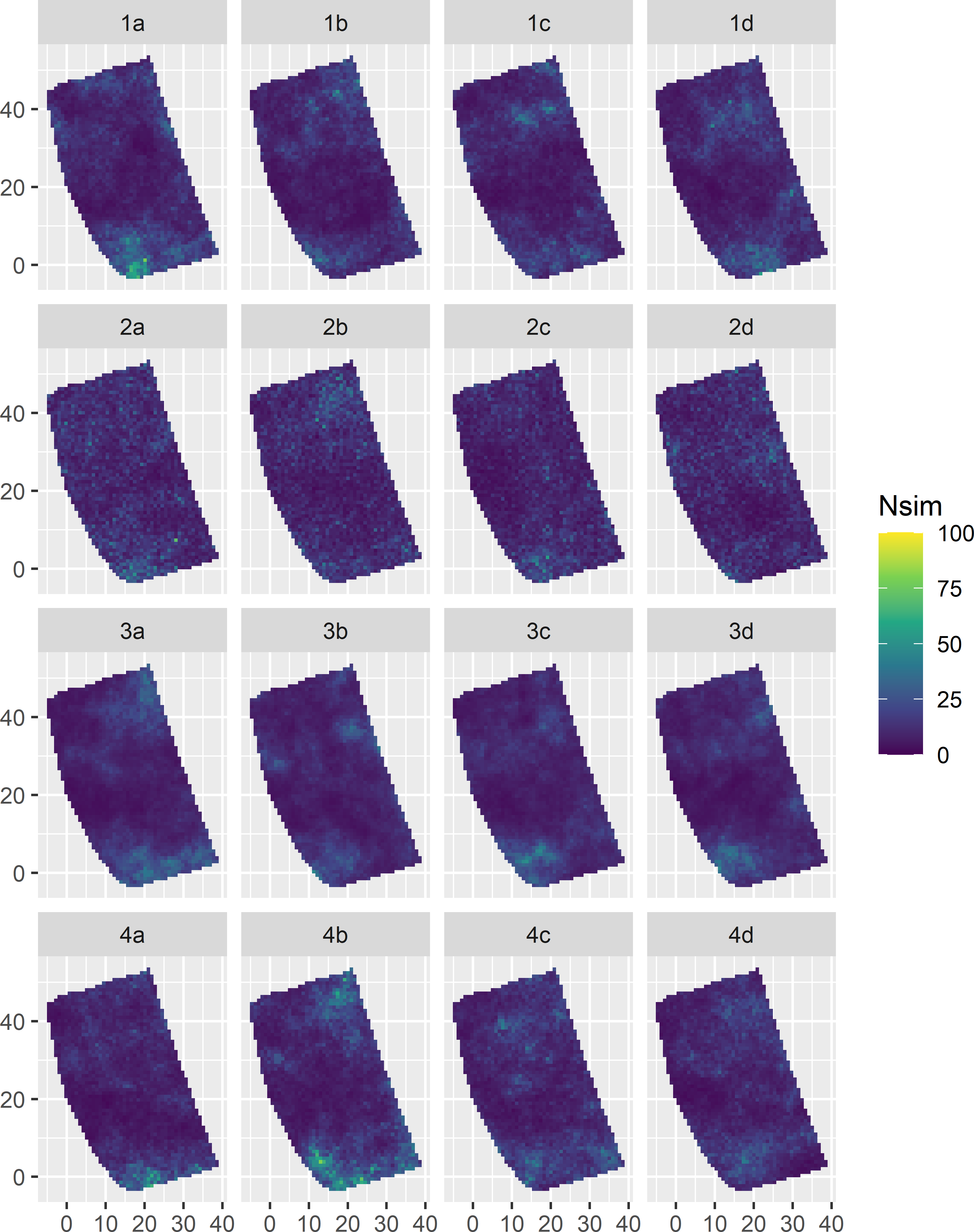
Figure 13.4: Maps of NO3-N of field Melle simulated with four semivariograms (rows). Each semivariogram is used to simulate four maps (columns a-d).
The sampling variances of the estimated mean of NO\(_3\)-N obtained with these 16 maps are shown below.
      a     b     c     d
1 1.364 0.831 0.878 0.847
2 1.379 1.151 0.991 1.162
3 0.669 0.594 0.522 0.530
4 0.932 1.949 0.878 0.739
The sampling variance shows quite strong variation among the maps. The frequency distribution of Figure 13.5 shows our uncertainty about the sampling variance, due to uncertainty about the semivariogram, and about the spatial distribution of NO\(_3\)-N within the agricultural field given the semivariogram and the available data from that field.
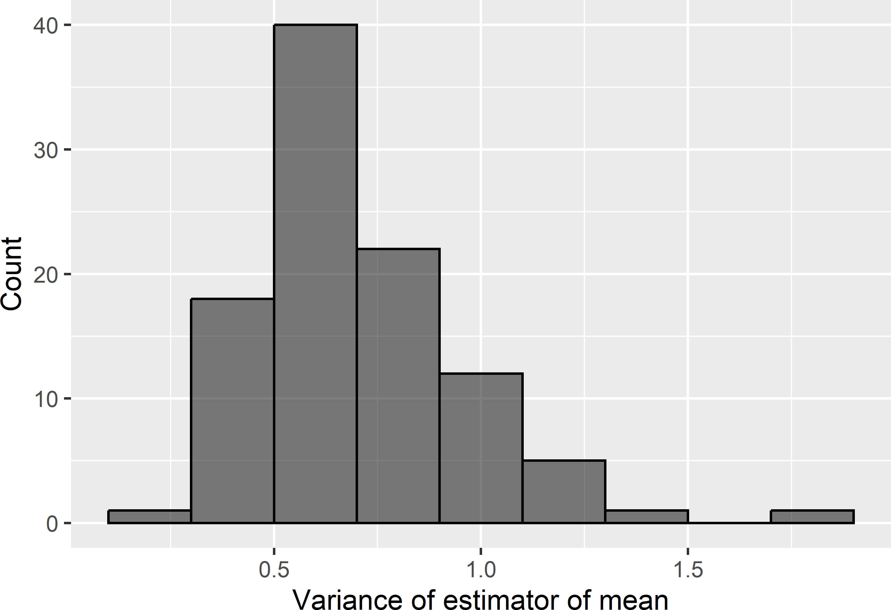
Figure 13.5: Frequency distribution of simulated sampling variances of the \(\pi\) estimator of the mean of NO3-N of field Melle, for stratified simple random sampling, using 25 compact geostrata of equal size, and one point per stratum.
As a model-based prediction of the sampling variance, we can take the mean or the median of the sampling variances over all 100 \(\times\) 100 simulated maps, which are equal to 0.728 (dag kg-1) and 0.666 (dag kg-1), respectively. If we want to be more safe, we can take a high quantile, e.g., the P90 of this distribution as the predicted sampling variance, which is equal to 1.100 (dag kg-1).
I used the 30 available NO\(_3\)-N data as conditioning data in geostatistical simulation. Unconditional simulation is recommended if we cannot rely on the quality of the legacy data, for instance due to a temporal change in lnN since the time the legacy data have been observed. For NO\(_3\)-N this might well be the case. I believe that, although the effect of 30 observations on the simulated fields and on the uncertainty distribution of the sampling variance will be very small, one still may prefer unconditional simulation. With unconditional simulation, we must assign the model-mean \(\mu\) to argument beta of function krige. The estimated model-mean can be estimated by generalised least squares, see function ll above.
13.2 Model-based optimisation of spatial strata
In this section a spatial stratification method is described that uses model predictions of the study variable as a stratification variable. As opposed to cum-root-f stratification, this spatial stratification method accounts for errors in the predictions, as well as for spatial correlation of the prediction errors (de Gruijter, Minasny, and McBratney 2015).
The Julia package Ospats is an implementation of this stratification method. In Ospats the stratification is optimised through iterative reallocation of the raster cells to the strata. Recently, this stratification method was implemented in the package SamplingStrata (Giulio Barcaroli (2014), G. Barcaroli et al. (2020)). However, the algorithm used to optimise the strata differs from that in Ospats. In SamplingStrata the stratification is optimised by optimising the bounds (splitting points) on the stratification variable with a genetic algorithm. Optimisation of the strata through optimisation of the bounds on the stratification variable necessarily leads to non-overlapping strata, while with iterative reallocation the strata may overlap, i.e., when the strata are sorted on the mean of the stratification variable, the upper bound of a stratum can be larger than the lower bound of the next stratum. As argued by de Gruijter, Minasny, and McBratney (2015) optimisation of strata through optimisation of the stratum bounds can be suboptimal. On the other hand, optimisation of the stratum bounds needs fewer computations and therefore is quicker.
The situation considered in this section is that prior data are available, either from the study area itself or from another similar area, that can be used to fit a linear regression model for the study variable, using one or more quantitative covariates and/or factors as predictors. These predictors must be available in the study area so that the fitted model can be used to map the study variable in the study area. We wish to collect more data by stratified simple random sampling, to be used in design-based estimation of the population mean or total of the study variable. The central research question then is how to construct these strata.
Recall the variance estimator of the mean estimator for stratified simple random sampling (Equations (4.4) and (4.5)):
\[\begin{equation} V\!\left(\hat{\bar{z}}\right)=\sum\limits_{h=1}^{H}w_{h}^{2} \frac{S^2_h(z)}{n_h}\;. \tag{13.9} \end{equation}\]
Plugging the stratum sample sizes under optimal allocation (Equation (4.17)) into Equation (13.9) yields
\[\begin{equation} V\!\left(\hat{\bar{z}}\right)=\frac{1}{n}\left(\sum\limits_{h=1}^{H}w_h S_h(z) \sqrt{c_h} \sum_{h=1}^H \frac{w_h S_h(z)}{\sqrt{c_h}}\right)\;. \tag{13.10} \end{equation}\]
So, given the total sample size \(n\), the variance of the estimator of the mean is minimal when the criterion
\[\begin{equation} O = \sum\limits_{h=1}^{H}w_h S_h(z) \sqrt{c_h} \sum_{h=1}^H \frac{w_h S_h(z)}{\sqrt{c_h}} \tag{13.11} \end{equation}\]
is minimised.
Assuming that the costs are equal for all population units, so that the mean costs are the same for all strata, the minimisation criterion reduces to
\[\begin{equation} O = \left(\sum\limits_{h=1}^H w_h S_h(z)\right)^2\;. \tag{13.12} \end{equation}\]
In practice, we do not know the values of the study variable \(z\). de Gruijter, Minasny, and McBratney (2015) consider the situation where we have predictions of the study variable from a linear regression model: \(\hat{z} = z + \epsilon\), with \(\epsilon\) the prediction error. So, this implies that we do not know the population standard deviations within the strata, \(S_h(z)\) of Equation (13.10). What we do have are the stratum standard deviations of the predictions of \(z\): \(S_h(\hat{z})\). With many statistical models, such as regression and kriging models, the standard deviation of the predictions is smaller than that of the study variable: \(S_h(\hat{z}) < S_h(z)\). This is known as the smoothing or levelling effect.
The stratum standard deviations in the minimisation criterion are replaced by model-expectations of the stratum standard deviations, i.e., by model-based predictions of the stratum standard deviations, \(E_{\xi}[S_h(z)]\). This leads to the following minimisation criterion:
\[\begin{equation} E_{\xi}[O] = \left(\sum\limits_{h=1}^H w_h E_{\xi}[S_h(z)]\right)^2\;. \tag{13.13} \end{equation}\]
The stratum variances are predicted by
\[\begin{equation} E_{\xi}[S^2_h(z)]=\frac{1}{N^2_h}\sum_{i=1}^{N_h-1}\sum_{j=i+1}^{N_h}E_{\xi}[d^2_{ij}]\;, \end{equation}\]
with \(d^2_{ij} = (z_i-z_j)^2\) the squared difference of the study variable values at two nodes of a discretisation grid. The model-expectation of the squared differences are equal to
\[\begin{equation} E_{\xi}[d^2_{ij}] = (\hat{z}_i-\hat{z}_j)^2+S^2(\epsilon_i)+S^2(\epsilon_j)-2S^2(\epsilon_i,\epsilon_j) \tag{13.14} \;, \end{equation}\]
with \(S^2(\epsilon_i)\) the variance of the prediction error at node \(i\) and \(S^2(\epsilon_i,\epsilon_j)\) the covariance of the prediction errors at nodes \(i\) and \(j\). The authors then argue that for smoothers, such as kriging and regression, the first term must be divided by the squared correlation coefficient \(R^2\):
\[\begin{equation} E_{\xi}[d^2_{ij}] = \frac{(\hat{z}_i-\hat{z}_j)^2}{R^2}+S^2(\epsilon_i)+S^2(\epsilon_j)-2S^2(\epsilon_i,\epsilon_j) \;. \tag{13.15} \end{equation}\]
The predicted stratum standard deviations are approximated by the square root of Equation (13.15). Plugging these model-based predictions of the stratum standard deviations into the minimisation criterion, Equation (13.12), yields
\[\begin{equation} E_{\xi}[O] = \frac{1}{N} \sum\limits_{h=1}^H \left( \sum_{i=1}^{N_h-1}\sum_{j=i+1}^{N_h}\frac{(\hat{z}_i-\hat{z}_j)^2}{R^2}+S^2(\epsilon_i)+S^2(\epsilon_j)-2S^2(\epsilon_i,\epsilon_j) \right)^{1 / 2}\;. \tag{13.16} \end{equation}\]
Optimal spatial stratification with package SamplingStrata is illustrated with a survey of the SOM concentration (g kg-1) in the topsoil (A horizon) of Xuancheng (China). Three samples are available. These three samples are merged. The total number of sampling points is 183. This sample is used to fit a simple linear regression model for the SOM concentration, using the elevation of the surface (dem) as a predictor. Function lm of the stats package is used to fit the simple linear regression model.
In fitting a linear regression model, we assume that the relation is linear, the residual variance is constant (independent of the fitted value), and the residuals have a normal distribution. These assumptions are checked with a scatter plot of the residuals against the fitted value and a Q-Q plot, respectively (Figure 13.6).

Figure 13.6: Scatter plot of residuals against fitted value and Q-Q plot of residuals, for a simple linear regression model of the SOM concentration in Xuancheng, using elevation as a predictor.
The scatter plot shows that the first assumption is realistic. No pattern can be seen: at all fitted values, the residuals are scattered around the horizontal line. However, the second and third assumptions are questionable: the residual variance clearly increases with the fitted value, and the distribution of the residuals has positive skew, i.e., it has a long upper tail. There clearly is some evidence that these two assumptions are violated. Possibly these problems can be solved by fitting a model for the natural log of the SOM concentration.
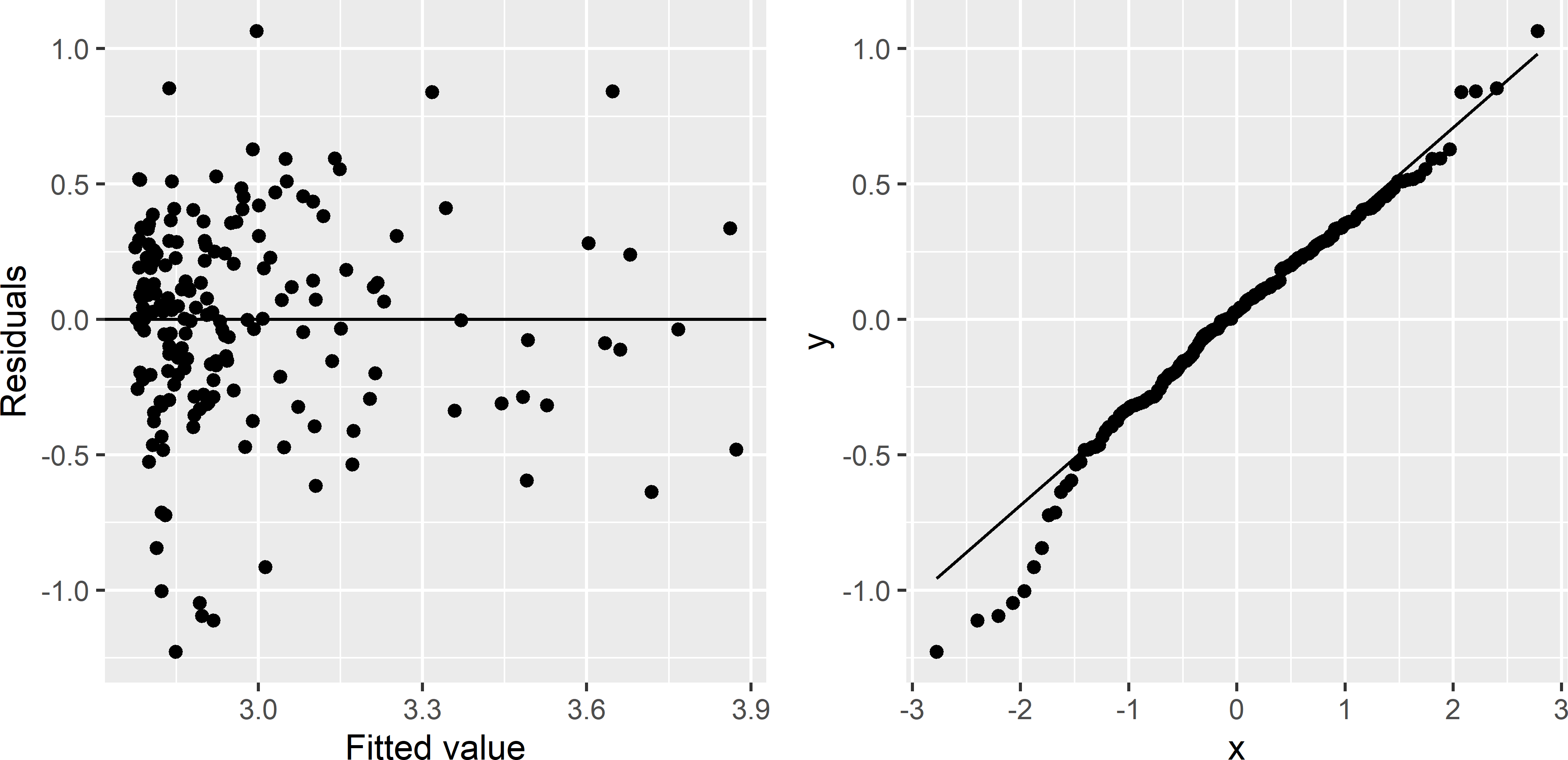
Figure 13.7: Scatter plot of residuals against fitted value and Q-Q plot of residuals, for a simple linear regression model of the natural log of the SOM concentration in Xuancheng, using elevation as a predictor.
The variance of the residuals is more constant (Figure 13.7), and the Q-Q plot is improved, although we now have too many strong negative residuals for a normal distribution. I proceed with the model for natural-log transformed SOM (lnSOM). The fitted linear regression model is used to predict lnSOM at the nodes of a 200 m \(\times\) 200 m discretisation grid.
res <- predict(lm_lnSOM, newdata = as(grdXuancheng, "data.frame"), se.fit = TRUE)
grdXuancheng <- within(grdXuancheng, {
  lnSOMpred <- res$fit; varpred <- res$se.fit^2})
The predictions and their standard errors are shown in Figure 13.8.
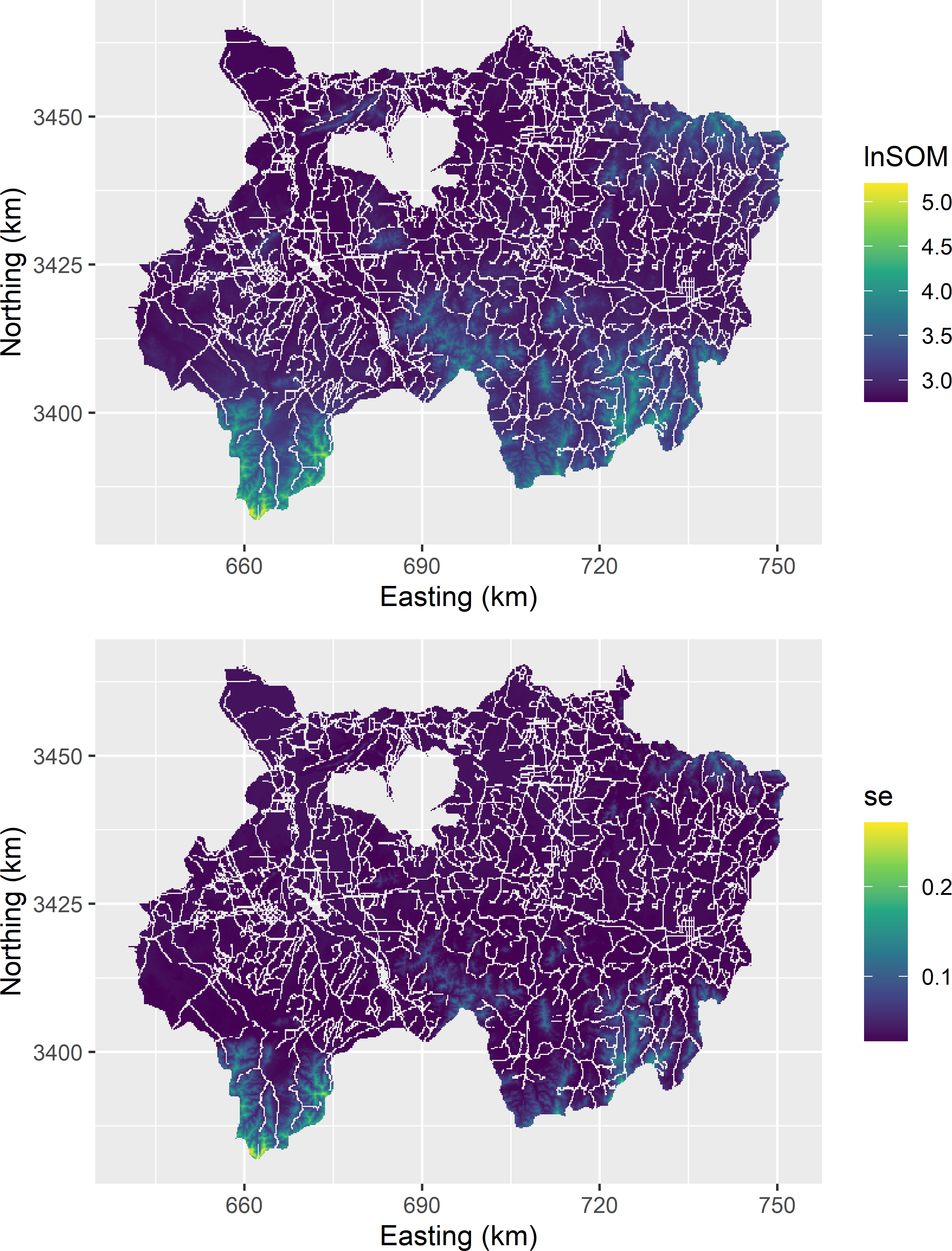
Figure 13.8: Predicted natural log of the SOM concentration (g kg-1) in the topsoil of Xuancheng and the standard error (se) of the predictor, obtained with a linear regression model with elevation as a predictor.
Let us check now whether the spatial structure of the study variable lnSOM is fully captured by the mean, modelled as a linear function of elevation. This can be checked by estimating the semivariogram of the model residuals. If the semivariogram of the residuals is pure nugget (the semivariance does not increase with distance), then we can assume that the prediction errors are independent. In that case, we do not need to account for a covariance of the prediction errors in optimisation of the spatial strata. However, if the semivariogram does show spatial structure, we must account for a covariance of the prediction errors. Figure 13.9 shows the sample semivariogram of the residuals computed with function variogram of package gstat.
library(gstat)
sampleXuancheng <- sampleXuancheng %>%
  mutate(s1 = s1 / 1000, s2 = s2 / 1000)
coordinates(sampleXuancheng) <- ~ s1 + s2
vg <- variogram(lnSOM ~ dem, data = sampleXuancheng)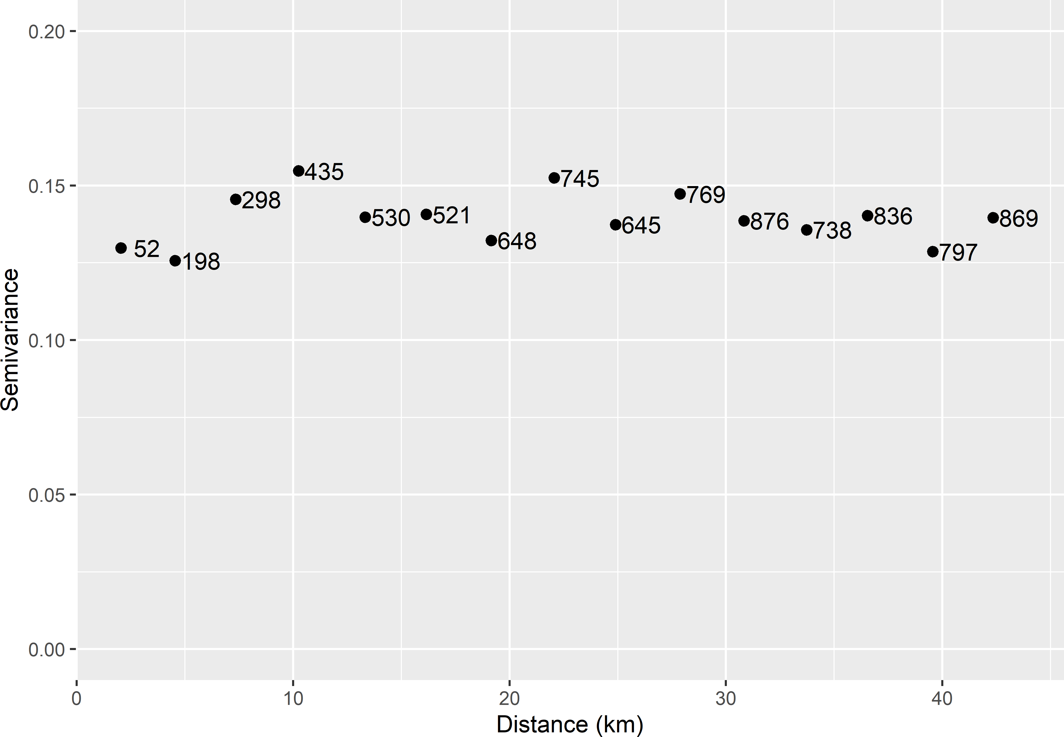
Figure 13.9: Sample semivariogram of the residuals of a simple linear regression model for the natural log of the SOM concentration in Xuancheng. Numbers refer to point-pairs used in computing semivariances.
The sample semivariogram does not show much spatial structure, but the first two points in the semivariogram have somewhat smaller values. This indicates that the residuals at two close points, say, \(<\pm 5\) km, are not independent, whereas if the distance between the two points \(>\pm 5\) km, they are independent. This spatial dependency of the residuals can be modelled, e.g., by an exponential function. The exponential semivariogram has three parameters, the nugget variance \(c_0\), the partial sill \(c_1\), and the distance parameter \(\phi\). The total number of model parameters now is five: two regression coefficients (intercept and slope for elevation) and three semivariogram parameters. All five parameters can best be estimated by restricted maximum likelihood, see Subsection 21.5.2. Table 13.1 shows the estimated regression coefficients and semivariogram parameters. Up to a distance of about three times the estimated distance parameter \(\phi\), which is about 8 km, the residuals are spatially correlated; beyond that distance, they are hardly correlated anymore.
| Int | dem | Nugget | Partial sill | Distance parameter (km) |
|---|---|---|---|---|
| 2.771 | 0.00222 | 0.085 | 0.061 | 2.588 |
We conclude that the errors in the regression model predictions are not independent, although the correlation will be weak in this case, and that we must account for this correlation in optimising the spatial strata.
The discretisation grid with predicted lnSOM consists of 115,526 nodes. These are too many for function optimStrata. The grid is therefore thinned to a grid with a spacing of 800 m \(\times\) 800 m, resulting in 7,257 nodes.
The first step in optimisation of spatial strata with package SamplingStrata is to build the sampling frame with function buildFrameSpatial. Argument X specifies the stratification variables, and argument Y specifies the study variables. In our case, we have only one stratification variable and one study variable, and these are the same variable. Argument variance specifies the variance of the prediction error of the study variable. Variable dom is an identifier of the domain of interest of which we want to estimate the mean or total. I assign the value 1 to all population units, see code chunk below, which implies that the stratification is optimised for the entire population. If we have multiple domains of interest, the stratification is optimised for each domain separately.
Finally, as a preparatory step we must specify how precise the estimated mean should be. This precision must be specified in terms of the coefficient of variation (cv), i.e., the standard error of the estimated mean divided by the mean. I use a cv of 0.005. In case of multiple domains of interest and multiple study variables, a cv must be specified per domain and per study variable. This precision requirement is used to compute the sample size for Neyman allocation (Equation (4.16))9. The optimal stratification is independent of the precision requirement.
library(SamplingStrata)
subgrd$id <- seq_len(nrow(subgrd))
subgrd$dom <- rep(1, nrow(subgrd))
frame <- buildFrameSpatial(df = subgrd, id = "id", X = c("lnSOMpred"),
  Y = c("lnSOMpred"), variance = c("varpred"), lon = "x1", lat = "x2",
  domainvalue = "dom")
cv <- as.data.frame(list(DOM = "DOM1", CV1 = 0.005, domainvalue = 1))
The optimal spatial stratification can be computed with function optimStrata, with argument method = "spatial". The \(R^2\) value of the linear regression model, used in the minimisation criterion (Equation (13.16)), can be specified with argument fitting.
Arguments range and kappa are parameters of an exponential semivariogram, needed for computing the covariance of the prediction errors. Function optimStrata uses an extra parameter in the exponential semivariogram: \(c_0+c_1\mathrm{exp}(-\kappa h/\phi)\). So, for the usual exponential semivariogram (Equation (21.13)) kappa equals 1.
res <- optimStrata(
  framesamp = frame, method = "spatial", errors = cv, nStrata = 5,
  fitting = 1, range = c(vgm_REML$phi), kappa = 1, showPlot = FALSE)
A summary of the optimised strata can be obtained with function summaryStrata.
  Domain Stratum Population Allocation SamplingRate Lower_X1 Upper_X1
1      1       1       3090         12     0.004035 2.767950 2.862539
2      1       2       1931         10     0.005087 2.864846 2.991733
3      1       3       1133         10     0.008555 2.994040 3.215515
4      1       4        769         11     0.014398 3.217822 3.600789
5      1       5        334         11     0.033443 3.605403 5.098052
In the next code chunk, it is checked whether the coefficient of variation is indeed equal to the desired value of 0.005.
strata <- res$aggr_strata
framenew <- res$framenew
N_h <- strata$N
w_h <- N_h / sum(N_h)
se <- sqrt(sum(w_h^2 * strata$S1^2 / strata$SOLUZ))
se / mean(framenew$Y1)
[1] 0.005033349The coefficient of variation can also be computed with function expected_CV.
     cv(Y1)
DOM1  0.005
Figure 13.10 shows the optimised strata. I used the stratum bounds in data.frame smr_strata, to compute the stratum for all raster cells of the original 200 m \(\times\) 200 m grid.
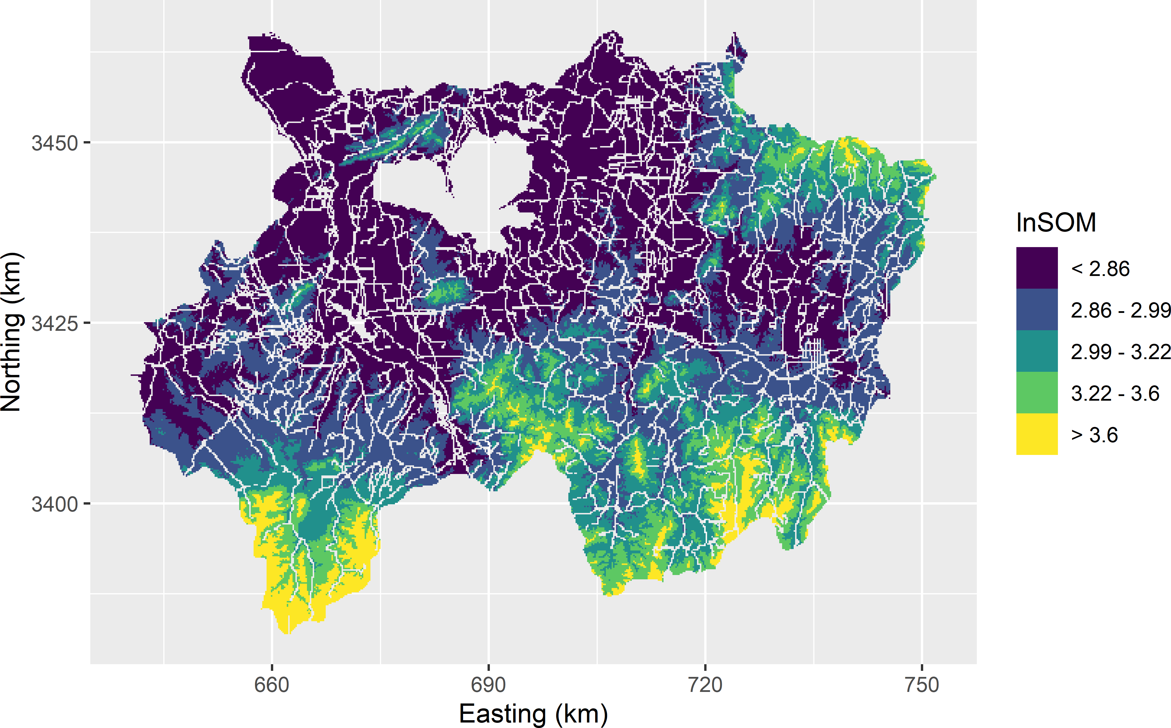
Figure 13.10: Model-based optimal strata for estimating the mean of the natural log of the SOM concentration in Xuancheng.
References
For multivariate stratification, i.e., stratification with multiple study variables, Bethel allocation is used to compute the required sample size.↩︎