Chapter 15 Repeated sample surveys for monitoring population parameters
The previous chapters are all about sampling to estimate population parameters at a given time. The survey is done in a relatively short period of time, so that we can safely assume that the study variable has not changed during that period. This chapter is about repeating the sample survey two or more times, to estimate, for instance, a temporal change in a population parameter. Sampling locations are selected by probability sampling, by any design type. In most cases, sampling times are not selected randomly, but purposively. For instance, to monitor the carbon stock in the soil of a country, we may decide to repeat the survey after five years, in the same season of the year as the first survey.
15.1 Space-time designs
An overview of space-time designs is presented by de Gruijter et al. (2006). Five of these designs are schematically shown in Figure 15.1. With repeated sampling in two-dimensional space, there are three dimensions: two spatial dimensions and one time dimension. Sampling locations shown in Figure 15.1 are selected by simple random sampling, but this is not essential for the space-time designs.
In the static-synchronous (SS) design, referred to as a pure panel by Fuller (1999), all sampling locations selected in the first survey are revisited in all subsequent surveys. On the contrary, in an independent synchronous (IS) design, a probability sample is selected in each survey independently from the samples selected in the previous surveys. The serially alternating (SA) design is a compromise between an SS and an IS design. The sample selected in the first survey is revisited in the third survey. The sample of the second survey is selected independently from the sample of the first survey, and these locations are revisited in the fourth survey. In this case, the period of revisits is two, i.e., two sampling intervals between consecutive surveys, but this can also be increased. For instance, with a period of three, three samples are selected, independently from each other, for the first three surveys, and these samples are revisited in subsequent surveys.
Two other compromise designs are a supplemented panel (SP) design and a rotating panel (RP) design. In an SP design only a subset of the sampling locations of the first survey is revisited in the subsequent surveys. These are the permanent sampling locations observed in all subsequent surveys. The permanent sampling locations are supplemented by samples that are selected independently from the samples in the previous surveys. In Figure 15.1, half of the sampling locations (ten locations) is permanent (panel a), i.e., revisited in all surveys, but the proportion of permanent sampling locations can be smaller or larger and, if prior information on the variation in space and time is available, even can be optimised for estimating the current mean. Also in an RP design, sampling units of the previous survey are partially replaced by new units. The difference with an SP design is that there are no permanent sampling units, i.e., no units observed in all surveys. All sampling units are sequentially rotated out and in again at the subsequent sampling times.
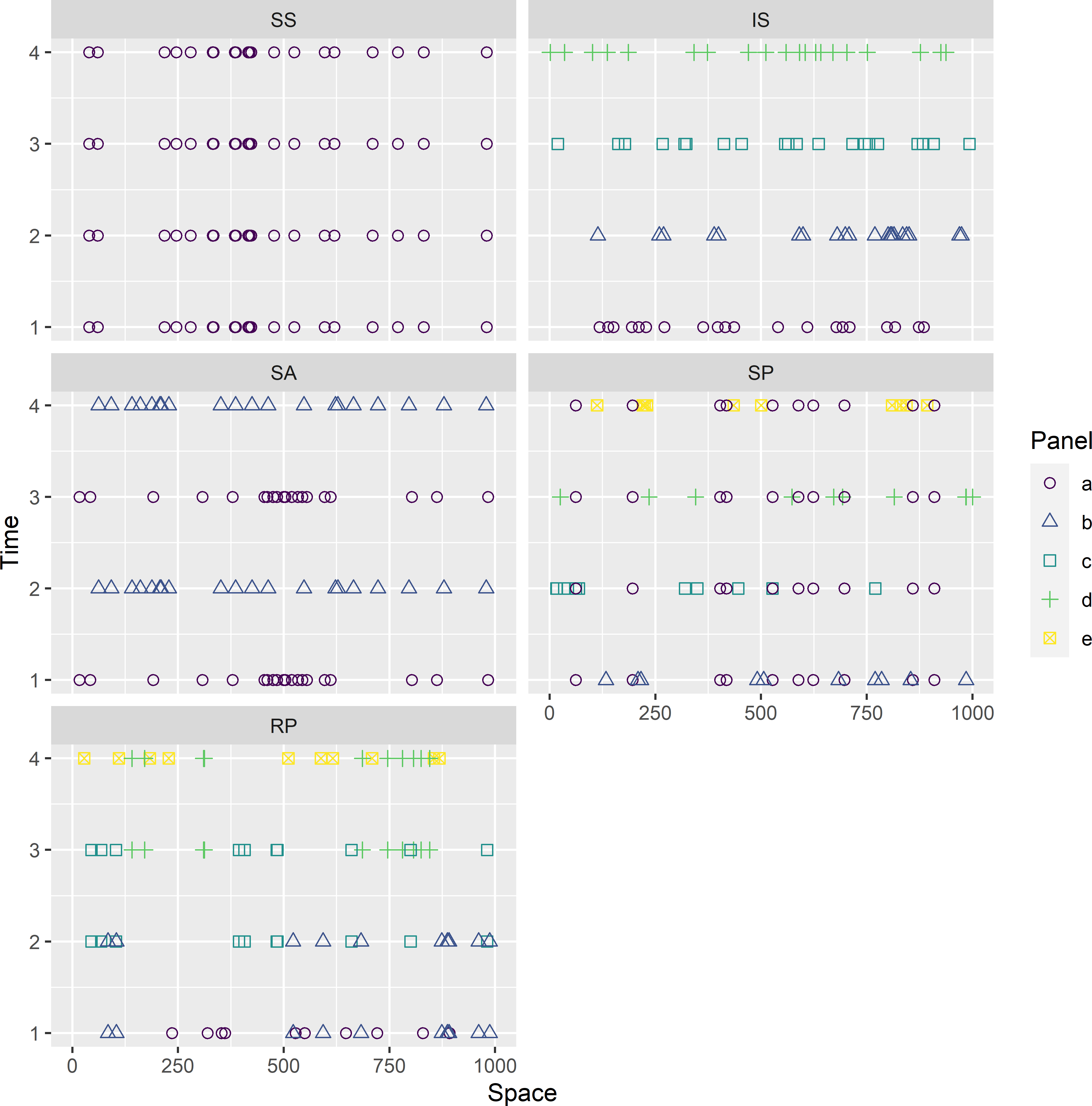
Figure 15.1: Space-time designs for monitoring population parameters. The sampling locations in 2D are plotted in one dimension, along the horizontal axis. A selected unit along this axis actually represents a sampling location in 2D. Twenty sampling locations are selected by simple random sampling. SS: static-synchronous design; IS: independent synchronous design; SA: serially alternating design; SP: supplemented panel design; RP: rotating panel design.
In Figure 15.1 the shape and colour of the symbols represent a panel. A panel is a group of sampling locations that is observed in the same surveys. In the SS design, there is only one panel. All locations are observed in all surveys, so all locations are in the same panel. In the IS design, there are as many panels as there are surveys. In the SA design with a period of two, the number of panels equals the number of surveys divided by two. In these three space-time designs (SS, IS, and SA), all sampling locations of a given survey are in the same panel. This is not the case in the SP and RP designs. In Figure 15.1 in each survey, two panels are observed. In the SP sample, there is one panel of permanent sampling locations (pure panel part of sample) and another panel of swarming sampling locations observed in one survey only. In the RP sample of Figure 15.1, the sampling locations are observed in two consecutive surveys; however, this number can be increased. For instance, in an ‘in-for-three’ rotational sample (McLaren and Steel 2001) the sampling locations stay in the sample for three consecutive surveys. The number of panels per sampling time is then three. Also, similar to an SA design, in an IS, SP, and RP design we may decide after several surveys to stop selecting new sampling locations and to revisit existing locations. The concept of panels is needed hereafter in estimating space-time population parameters.
15.2 Space-time population parameters
The data of repeated surveys can be used to estimate various parameters of the space-time universe. I will focus on the mean as a parameter, but estimation of a total or proportion is straightforward, think for instance of the total amount of greenhouse gas emissions from the soil in a given study area during some period. This chapter shows how to estimate the current mean, i.e., the population mean (spatial mean) in the last survey, the change of the mean between two surveys, the temporal trend of the mean, and the space-time mean. The current mean need not be defined here as only one survey (one sampling time) is involved in this parameter, so that the definition in Subsection 1.1.1 is also relevant here.
The change of the mean is defined as the spatial mean at a given survey minus this mean at an earlier survey. For finite populations, the definition is
\[\begin{equation} \bar{d}_{ab}=\frac{1}{N}\left(\sum_{k=1}^N z_k(t_b) -\sum_{k=1}^N z_k(t_a) \right)=\frac{1}{N}\sum_{k=1}^N d_{abk}\;, \tag{15.1} \end{equation}\]
with \(d_{abk}\) the change of the study variable in the period between time \(t_a\) and \(t_b\) for unit \(k\). For infinite populations, the sums are replaced by integrals:
\[\begin{equation} \bar{d}_{ab}=\frac{1}{A}\left(\int_{\mathbf{s} \in \mathcal{A}} z(\mathbf{s},t_b) \;\mathrm{d}\mathbf{s}-\int_{\mathbf{s} \in \mathcal{A}} z(\mathbf{s},t_a) \;\mathrm{d}\mathbf{s}\right)=\frac{1}{A}\int_{\mathbf{s} \in \mathcal{A}}d_{ab}(\mathbf{s})\;, \tag{15.2} \end{equation}\]
with \(d_{ab}(\mathbf{s})\) the change of the study variable in the period between time \(t_a\) and \(t_b\) at location \(\mathbf{s}\).
With more than two surveys, an interesting population parameter is the average change per time unit of the mean, referred to as the temporal trend of the spatial mean. It is defined as a linear combination of the spatial means at the sampling times (Breidt and Fuller 1999):
\[\begin{equation} b=\sum_{j=1}^R w_j \bar{z}_j \;, \tag{15.3} \end{equation}\]
with \(R\) the number of sampling times, \(\bar{z}_j\) the spatial mean at time \(t_j\), and weights \(w_j\) equal to
\[\begin{equation} w_j = \frac{t_j-\bar{t}}{\sum_{j=1}^R(t_j-\bar{t})^2} \;, \tag{15.4} \end{equation}\]
with \(\bar{t}\) the mean of the sampling times.
A space-time mean can be defined as the average of the spatial means at the sampling times. In this definition, the temporal universe is discrete and restricted to the sampling times. The target universe consists of a finite set of spatial populations:
\[\begin{equation} \bar{\bar{z}}_{\mathcal{U}}=\frac{1}{R} \sum_{j=1}^R \bar{z_j}\;. \tag{15.5} \end{equation}\]
Alternatively, a space-time mean for a continuous temporal universe \(\mathcal{T}\) is defined as
\[\begin{equation} \bar{\bar{z}}_{\mathcal{U}} = \frac{1}{T}\int_{t \in \mathcal{T}}\bar{z}_t\;, \tag{15.6} \end{equation}\]
with \(T\) the length of the monitoring period and \(\bar{z}_t\) the spatial mean at time \(t\).
15.3 Design-based generalised least squares estimation of spatial means
Rotational sampling has a long tradition in agronomy, forestry, and in social studies. Early papers on how sample data from previous times can be used to increase the precision of estimates of the current mean are Jessen (1942), Patterson (1950), Ware and Cunia (1962), and Woodruff (1963). Gurney and Daly (1965) developed general theory for these estimators, which I will present now.
In overlapping samples such as an SP and an RP sample, we may define one estimate of a spatial mean per ‘panel’. These panel-specific estimates of the mean at a given sampling time, based on observations at that time only, are referred to as elementary estimates.
The essence of the estimation method described in this section is to estimate the spatial mean at a given time point as a weighted average of the elementary estimates of all time points, with the weights determined by the variances and covariances of the elementary estimates. Collecting all elementary estimates of the spatial means of the different sampling times in vector \(\hat{\mathbf{z}}\), we can write
\[\begin{equation} \hat{\mathbf{z}}=\mathbf{X} \mathbf{z} + \mathbf{e} \;, \tag{15.7} \end{equation}\]
with \(\mathbf{z}\) the vector of true spatial means \(\bar{z}(t_1), \dots ,\bar{z}(t_R)\) at the \(R\) sampling times, \(\mathbf{X}\) the (\(P \times R\)) design matrix with zeroes and ones that selects the appropriate elements from \(\mathbf{z}\) (\(P\) is the total number of elementary estimates), and \(\mathbf{e}\) the \(P\)-vector of sampling errors with variance-covariance matrix \(\mathbf{C}\). With unbiased elementary estimators, the expectation of \(\mathbf{e}\) is a vector with zeroes.
With an SS, IS, and SA design, the design matrix \(\mathbf{X}\) is the identity matrix of size \(R\), i.e., an \(R \times R\) square matrix with ones on the diagonal and zeroes in all off-diagonal entries. For the SP design of Figure 15.1, the design matrix \(\mathbf{X}\) is
\[\begin{equation} \mathbf{X}= \begin{bmatrix} 1 &0 &0 &0\\ 0 &1 &0 &0\\ 0 &0 &1 &0\\ 0 &0 &0 &1\\ 1 &0 &0 &0\\ 0 &1 &0 &0\\ 0 &0 &1 &0\\ 0 &0 &0 &1 \end{bmatrix} \;. \tag{15.8} \end{equation}\]
The first four rows of this matrix are associated with the elementary estimates of the spatial means at the four sampling times, estimated from panel a, the panel with permanent sampling locations. Hereafter, this panel is referred to as the static-synchronous subsample. The remaining rows correspond to the elementary estimates from the other four panels, the swarming locations, hereafter referred to as the independent-synchronous subsamples. For the RP design of Figure 15.1, the design matrix equals
\[\begin{equation} \mathbf{X}= \begin{bmatrix} 1 &0 &0 &0\\ 1 &0 &0 &0\\ 0 &1 &0 &0\\ 0 &1 &0 &0\\ 0 &0 &1 &0\\ 0 &0 &1 &0\\ 0 &0 &0 &1\\ 0 &0 &0 &1 \end{bmatrix} \;. \tag{15.9} \end{equation}\]
The first two rows correspond to the two elementary estimates of the mean at time \(t_1\) from panels a and b, the third and fourth rows correspond to the elementary estimate at time \(t_2\) from panels b and c, respectively, etc.
The minimum variance linear unbiased estimator (MVLUE) of the spatial means at the different times is the design-based generalised least squares (GLS) estimator (Binder and Hidiroglou 1988):
\[\begin{equation} \hat{\mathbf{z}}_{\mathrm{GLS}}=(\mathbf{X}^{\text{T}}\mathbf{C}^{-1}\mathbf{X})^{-1} \mathbf{X}^{\text{T}} \mathbf{C}^{-1} \hat{\mathbf{z}}\;. \tag{15.10} \end{equation}\]
To define matrix \(\mathbf{C}\) for the SP design in Figure 15.1, let \(\hat{\bar{z}}_{jp}\) denote the estimated mean at time \(t_j, j = 1,2,3,4\) in subsample \(p, p \in (a,b,c,d,e)\), with panel \(a\) the permanent sampling locations (SS subsample) and panels \(b,c,d,e\) the swarming sampling locations (IS subsamples). If the eight elementary estimates in \(\hat{\mathbf{z}}\) are ordered as (\(\hat{\bar{z}}_{1a},\hat{\bar{z}}_{2a},\hat{\bar{z}}_{3a},\hat{\bar{z}}_{4a},\hat{\bar{z}}_{1b},\hat{\bar{z}}_{2c},\hat{\bar{z}}_{3d},\hat{\bar{z}}_{4e}\)), the variance-covariance matrix \(\mathbf{C}\) equals
\[\begin{equation} \mathbf{C}= \begin{bmatrix} V_{1a} &C_{1,2} &C_{1,3} &C_{1,4} &0 &0 &0 &0 \\ C_{2,1} &V_{2a} &C_{2,3} &C_{2,4} &0 &0 &0 &0 \\ C_{3,1} &C_{3,2} &V_{3a} &C_{3,4} &0 &0 &0 &0 \\ C_{4,1} &C_{4,2} &C_{4,3} &V_{4a} &0 &0 &0 &0 \\ 0 &0 &0 &0 &V_{1b} &0 &0 &0 \\ 0 &0 &0 &0 &0 &V_{2c} &0 &0 \\ 0 &0 &0 &0 &0 &0 &V_{3d} &0 \\ 0 &0 &0 &0 &0 &0 &0 &V_{4e} \end{bmatrix} \;. \tag{15.11} \end{equation}\]
The covariances of the elementary estimates of the IS subsamples are zero because these are estimated from independently selected samples (off-diagonal elements in lower right (4 \(\times\) 4) submatrix). Also the covariances of the elementary estimates from the SS subsample and an IS subsample are zero for the same reason (upper right submatrix and lower left submatrix). The covariances of the four elementary estimates from the SS subsample are not zero because these are estimated from the same set of sampling locations.
Ordering the elementary estimates of the RP sample by the sampling times, the variance-covariance matrix equals
\[\begin{equation} \mathbf{C}= \begin{bmatrix} V_{1a} &0 &0 &0 &0 &0 &0 &0 \\ 0 &V_{1b} &C_{1,2} &0 &0 &0 &0 &0 \\ 0 &C_{2,1} &V_{2b} &0 &0 &0 &0 &0 \\ 0 &0 &0 &V_{2c} &C_{2,3} &0 &0 &0 \\ 0 &0 &0 &C_{3,2} &V_{3c} &0 &0 &0 \\ 0 &0 &0 &0 &0 &V_{3d} &C_{3,4} &0 \\ 0 &0 &0 &0 &0 &C_{4,3} &V_{4d} &0 \\ 0 &0 &0 &0 &0 &0 &0 &V_{4e} \end{bmatrix} \;. \tag{15.12} \end{equation}\]
Only the elementary estimates of the same panel are correlated, for instance the elementary estimates of the spatial means at times \(t_1\) and \(t_2\), estimated from panel b.
For the SA design of Figure 15.1 the variance-covariance matrix equals (there is only one estimate per time)
\[\begin{equation} \mathbf{C}= \begin{bmatrix} V_{1} &0 &C_{1,3} &0 \\ 0 &V_{2} &0 &C_{2,4} \\ C_{3,1} &0 &V_{3} &0 \\ 0 &C_{4,2} &0 &V_{4} \end{bmatrix} \;. \tag{15.13} \end{equation}\]
In practice, matrix \(\mathbf{C}\) in Equation (15.10) is unknown and is replaced by a matrix with design-based estimates of the variances and covariances of the elementary estimators. With simple random sampling with replacement from finite populations and simple random sampling of infinite populations, the variance of an elementary estimator of the spatial mean at a given time can be estimated by Equation (3.10). The covariance of the elementary estimators of the spatial means at two sampling times, using the data of the same panel, can be estimated by
\[\begin{equation} \widehat{C}_{ab} = \frac{\widehat{S^2}_{ab}}{m} \;, \tag{15.14} \end{equation}\]
with \(m\) the number of sampling locations in the panel and \(\widehat{S^2}_{ab}\) the estimated covariance of the study variable at times \(t_a\) and \(t_b\), estimated by
\[\begin{equation} \widehat{S^2}_{ab} = \frac{1}{m-1}\sum_{k=1}^m (z_{apk}-\hat{\bar{z}}_{ap})(z_{bpk}-\hat{\bar{z}}_{bp}) \;, \tag{15.15} \end{equation}\]
with \(z_{apk}\) the study variable of unit \(k\) in panel \(p\) at time \(t_a\) and \(\hat{\bar{z}}_{ap}\) the spatial mean at time \(t_a\) as estimated from panel \(p\).
The variances and covariances of the GLS estimators of the spatial means at the \(R\) sampling times can be estimated by
\[\begin{equation} \widehat{\mathbf{C}}(\hat{\mathbf{z}}_{\mathrm{GLS}}) = (\mathbf{X}^{\text{T}}\widehat{\mathbf{C}}^{-1}\mathbf{X})^{-1} \tag{15.16} \;. \end{equation}\]
Given the design-based GLS estimates of the spatial means at the different times, it is an easy job to compute the estimated change of the mean between two surveys, the estimated temporal trend of the mean, and the estimated space-time mean.
15.3.1 Current mean
As explained above, with the SS, IS, and SA designs, the design matrix \(\mathbf{X}\) is the identity matrix of size \(R\). From this it follows that for these space-time designs \(\hat{\mathbf{z}}_{\mathrm{GLS}}=\hat{\mathbf{z}}\), see Equation (15.10), and \(\mbox{Cov}(\hat{\mathbf{z}}_{\mathrm{GLS}})=\mbox{Cov}(\hat{\mathbf{z}})=\mathbf{C}\). In words, the GLS estimator of the spatial mean at a given time equals the usual \(\pi\) estimator of the mean at that time, and the variance-covariance matrix of the GLS estimators of the spatial means equals the variance-covariance matrix of the \(\pi\) estimators.
With SP and RP sampling in space-time, there is partial overlap between the samples at the different times, and so the samples at the previous times can be used to increase the precision of the estimated mean at the last time (current mean). The estimated current mean is simply the last element in \(\hat{\mathbf{z}}_{\mathrm{GLS}}\). The estimated variance of the estimator of the current mean is the element in the final row and final column of the variance-covariance matrix of the estimated spatial means (Equation (15.16)). These two space-time designs with partial replacement of sampling locations may yield a more precise estimate of the current mean than the other three space-time designs.
15.3.2 Change of the spatial mean
The change of the spatial mean between two sampling times can simply be estimated by subtracting the estimated spatial means at these two times. With the SS, IS, and SA designs, these means are estimated by the \(\pi\) estimators. With the SP and RP designs, the two spatial means are estimated by the GLS estimators. The variance of the estimator of the change can be estimated by the sum of the estimated variances of the spatial mean estimators at the two sampling times, minus two times the estimated covariance of the two estimators. The covariance is maximal when all sampling locations are revisited, leading to the most precise estimate of the change of the spatial mean. With SP and RP sampling, the covariance of the two spatial mean estimators is smaller, and so the variance of the change estimator is larger.
15.3.3 Temporal trend of the spatial mean
The temporal trend of the mean is estimated by the weighted average of the (GLS) estimated means at \(t_1,\dots ,t_R\), with weights equal to Equation (15.4):
\[\begin{equation} \hat{b}=\sum_{j=1}^R w_j \hat{\bar{z}}_{\mathrm{GLS},j} \;. \tag{15.17} \end{equation}\]
The variance of the estimator of the temporal trend can be estimated by
\[\begin{equation} \widehat{V}(\hat{b}) = \mathbf{w}^{\mathrm{T}}\widehat{\mathbf{C}}(\hat{\mathbf{z}}_{\mathrm{GLS}}) \mathbf{w}\;. \tag{15.18} \end{equation}\]
Brus and de Gruijter (2011) compared the space-time designs for estimating the temporal trend of the spatial means, under a first order autoregressive time-series model of the spatial means. The SS design performed best when the correlation is strong, say \(>0.8\). What is the best design depends amongst others on the strength of the correlation and the number of sampling times. A safe choice is an SA design. With strong positive correlation, say \(>0.9\), the SS design can be a good choice, but remarkably for weak positive correlation this design performed relatively poorly.
For an application of an SP design to estimate the temporal trend of the areal fractions of several vegetation types, see Brus et al. (2014). Sampling locations are selected by a design that spreads the locations evenly over the study area (systematic unaligned sampling, which is a modified version of systematic sampling).
15.3.4 Space-time mean
The space-time mean, as defined in Equation (15.5), can be estimated by the average of the (GLS) estimated spatial means at the \(R\) sampling times. The variance of this estimator can be estimated by Equation (15.18) using constant weights, equal to \(1/R\), for the \(R\) estimators of the mean. An IS design yields the most precise estimate of the space-time mean compared to the other space-time designs when the correlation of collocated measurements of the study variable is positive (Cochran 1977). With the other space-time designs, there is redundant information due to the revisits.
For design-based estimation of the space-time mean of a continuous temporal universe as defined in Equation (15.6), both the sampling locations and the sampling times must be selected by probability sampling. Figure 15.2 shows an SS sample and an IS sample of twenty locations and six times, where both locations and times are selected by simple random sampling.
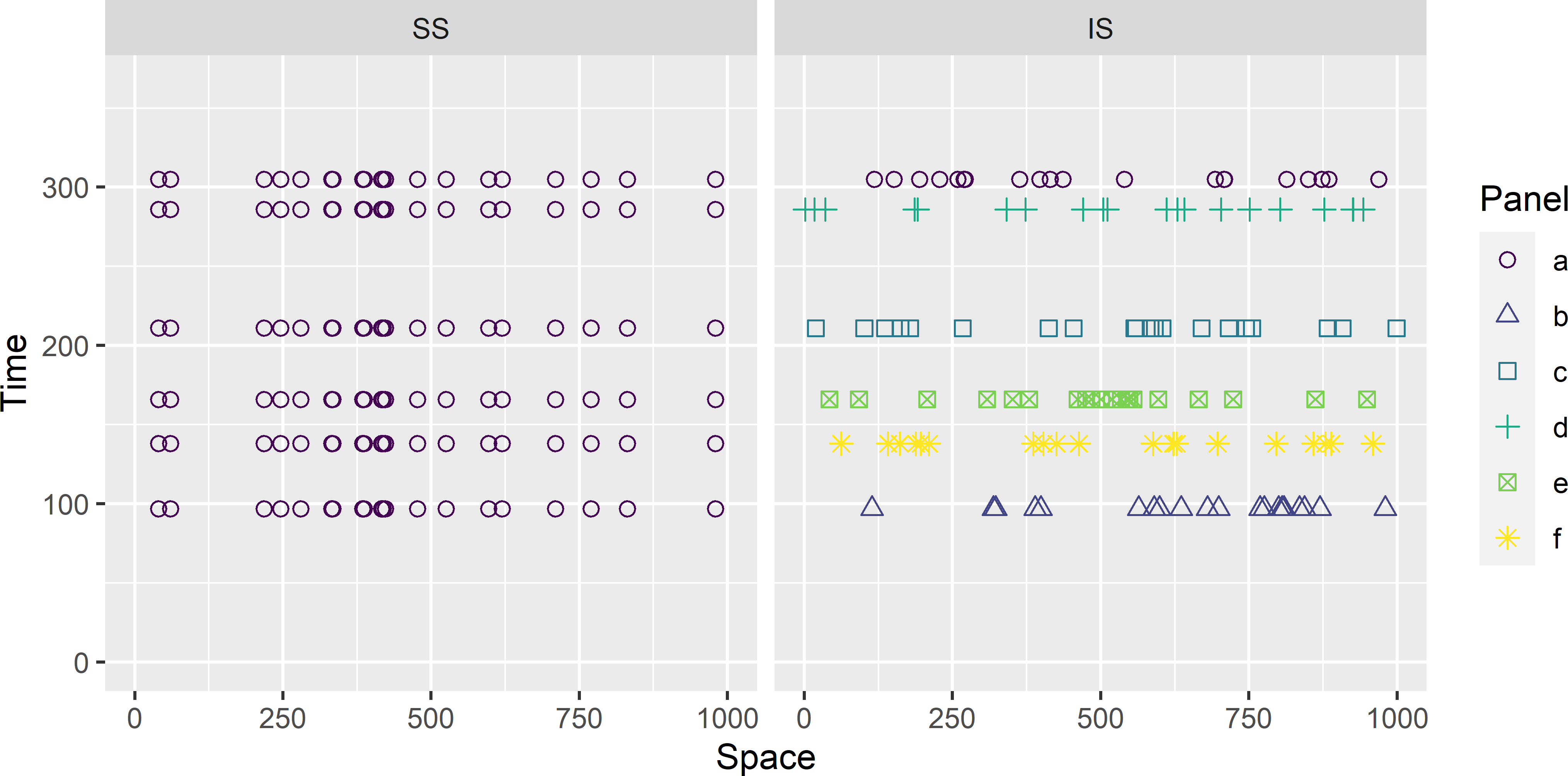
Figure 15.2: Space-time designs for estimating the space-time mean of a continuous temporal universe. Both locations and times are selected by simple random sampling. SS: static-synchronous design; IS: independent synchronous design.
An IS sample in which both locations and times are selected by probability sampling can be considered as a two-stage cluster random sample from a space-time universe (Chapter 7). The primary sampling units (PSUs) are the spatial sections of that universe (horizontal lines in Figure 15.2), the secondary sampling units (SSUs) are the sampling locations. The space-time mean can therefore be estimated by Equation (7.2), and its variance by Equation (7.7). For simple random sampling, both in space and in time, and a linear costs model \(C = c_0 + c_1n + c_2nm\) Equations (7.9) and (7.10) can be used to optimise the number of sampling times (PSUs, \(n\)) and the number of sampling locations (SSUs, \(m\)) per time. The pooled within-unit variance, \(S^2_\text{w}\), is in this case the time-averaged spatial variance of the study variable at a given time, and the between-unit variance, \(S^2_\text{b}\), is the variance of the spatial means over time.
Estimation of the space-time mean from an SS sample in which both locations and times are selected by probability sampling is the same as for an IS sample. However, estimation of the variance of the space-time mean estimator is more complicated. For the variance of the estimator of the space-time mean with an SS space-time design and simple random sampling of both locations and times, see equation (15.8) in de Gruijter et al. (2006). Due to the two-fold alignment of the sampling units, no unbiased estimator of the variance is available. The variance estimator of two-stage cluster sampling can be used to approximate the variance, but this variance estimator does not account for a possible temporal correlation of the estimated spatial means, resulting in an underestimation of the variance.
For an application of an IS design, to estimate the space-time mean of nutrients (nitrogen and phosphorous) in surface waters, see Brus and Knotters (2008) and Knotters and Brus (2010). In both applications, sampling times are selected by stratified simple random sampling, with periods of two months as strata. In Brus and Knotters (2008), sampling locations are selected by stratified simple random sampling as well.
15.4 Case study: annual mean daily temperature in Iberia
The space-time designs are illustrated with the annual mean air temperature at two metres above the earth surface (TAS) in Iberia for 2004, 2009, 2014, and 2019 (Subsection 1.3.4).
Sampling locations are selected by simple random sampling. The sample size is 100 locations per survey; so with four surveys we have 400 observations in total, but not with all space-time designs at 400 different sampling locations. In the next sections, I will show how a space-time sample with a given space-time design can be selected, and how the population parameters described in Section 15.2 can be estimated.
15.4.1 Static-synchronous design
Selecting an SS space-time sample, using simple random sampling as a spatial design, is straightforward. We can simply select a single simple random sample of size \(n=100\). The locations of this sample are observed at all times (Figure 15.3).
grd <- grdIberia %>%
  mutate(x = x / 1000,
         y = y / 1000)
set.seed(314)
n <- 100
units <- sample(nrow(grd), size = n, replace = TRUE)
mysample_SS <- grd[units, ]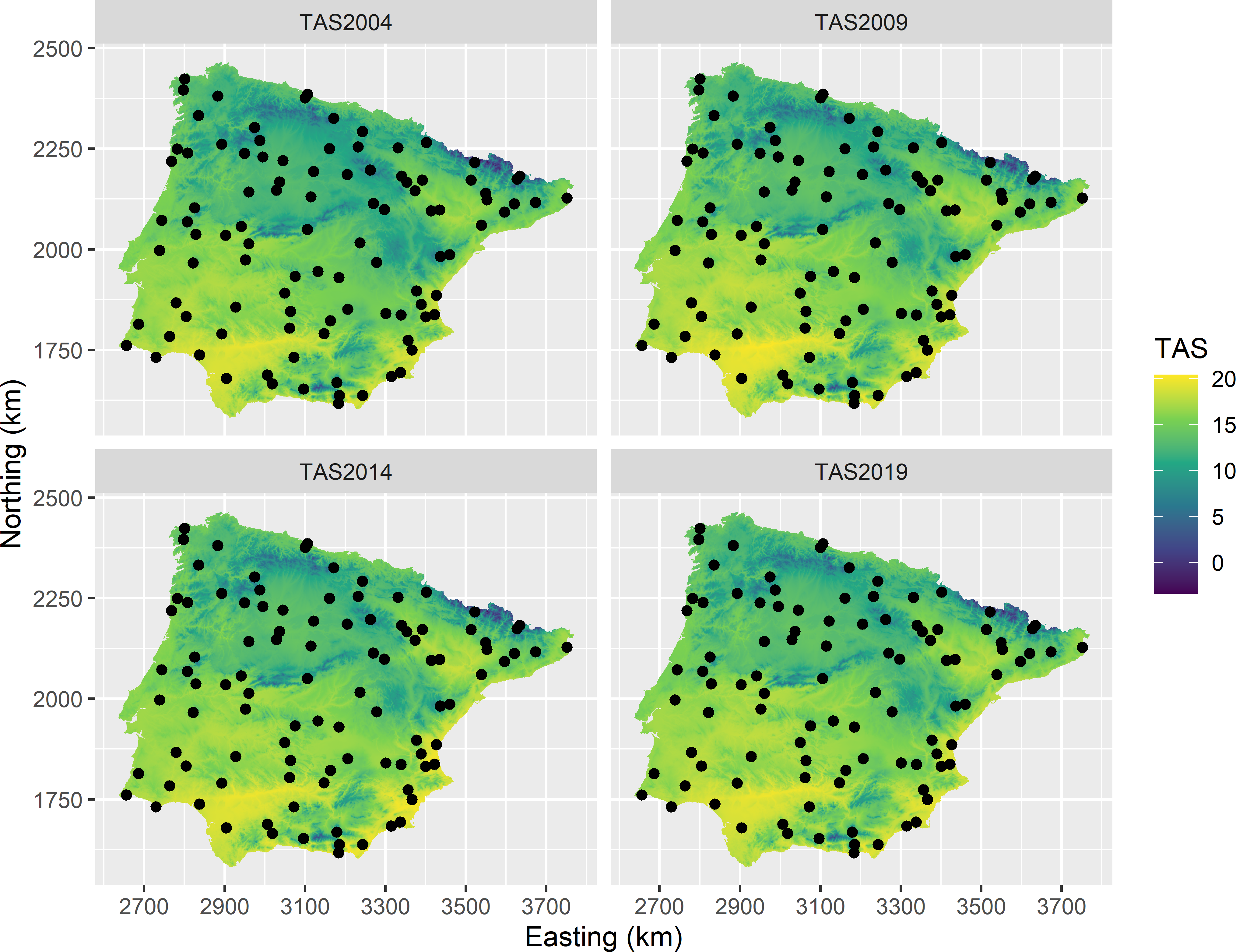
Figure 15.3: Static-synchronous space-time sample from Iberia. Locations are selected by simple random sampling.
The spatial means at the four times can be estimated by the sample means (Equation (3.2)), the variances of the mean estimators by Equation (3.10). The covariances of the estimators of the means at two different times can be estimated by Equation (15.14) with \(m\) equal to the sample size \(n\). The estimated current mean (the spatial mean at the fourth survey) and the estimated standard error of the estimator of the current mean can be simply extracted from the vector with estimated means and from the matrix with estimated variances and covariances.
mz <- apply(mysample_SS[, -c(1, 2)], MARGIN = 2, FUN = mean)
C <- var(mysample_SS[, -c(1, 2)]) / n
#current mean
mz_cur_SS <- mz[4]
se_mz_cur_SS <- sqrt(C[4, 4])
The change of the spatial mean from the first to the fourth survey can simply be estimated by subtracting the estimated spatial mean of the first survey from the estimated mean of the fourth survey. The standard error of this estimator can be estimated by the sum of the estimated variances of the two spatial mean estimators, minus two times the estimated covariance of the two mean estimators, and finally taking the square root.
The same estimates are obtained by defining a weight vector with values -1 and 1 for the first and last element, respectively, and 0 for the other two elements.
The temporal trend of the spatial means can be estimated much in the same way, but using a different vector with weights (Equation (15.4)).
t <- seq(from = 2004, to = 2019, by = 5)
w <- (t - mean(t)) / sum((t - mean(t))^2)
mz_trend_SS <- t(w) %*% mz
se_mz_trend_SS <- sqrt(t(w) %*% C %*% w)
The estimated temporal trend equals 0.0403\(^\circ\)C \(y^{-1}\), and the estimated standard error equals 0.0024794\(^\circ\)C \(y^{-1}\). Using t = 1:4 yields the estimated average change in annual mean temperature per five years.
          [,1]
[1,] 0.2016378
Using a constant weight vector with values 1/4 yields the estimated space-time mean and the standard error of the space-time mean estimator.
15.4.2 Independent synchronous design
To select an IS space-time sample with four sampling times, we simply select \(4n=400\) sampling locations. Figure 15.4 shows the selected IS space-time sample. A variable identifying the panel of the selected sampling units is added to the data frame.
units <- sample(nrow(grd), size = 4 * n, replace = TRUE)
mysample_IS <- grd[units, ]
mysample_IS$panel <- rep(c("a", "b", "c", "d"), each = n)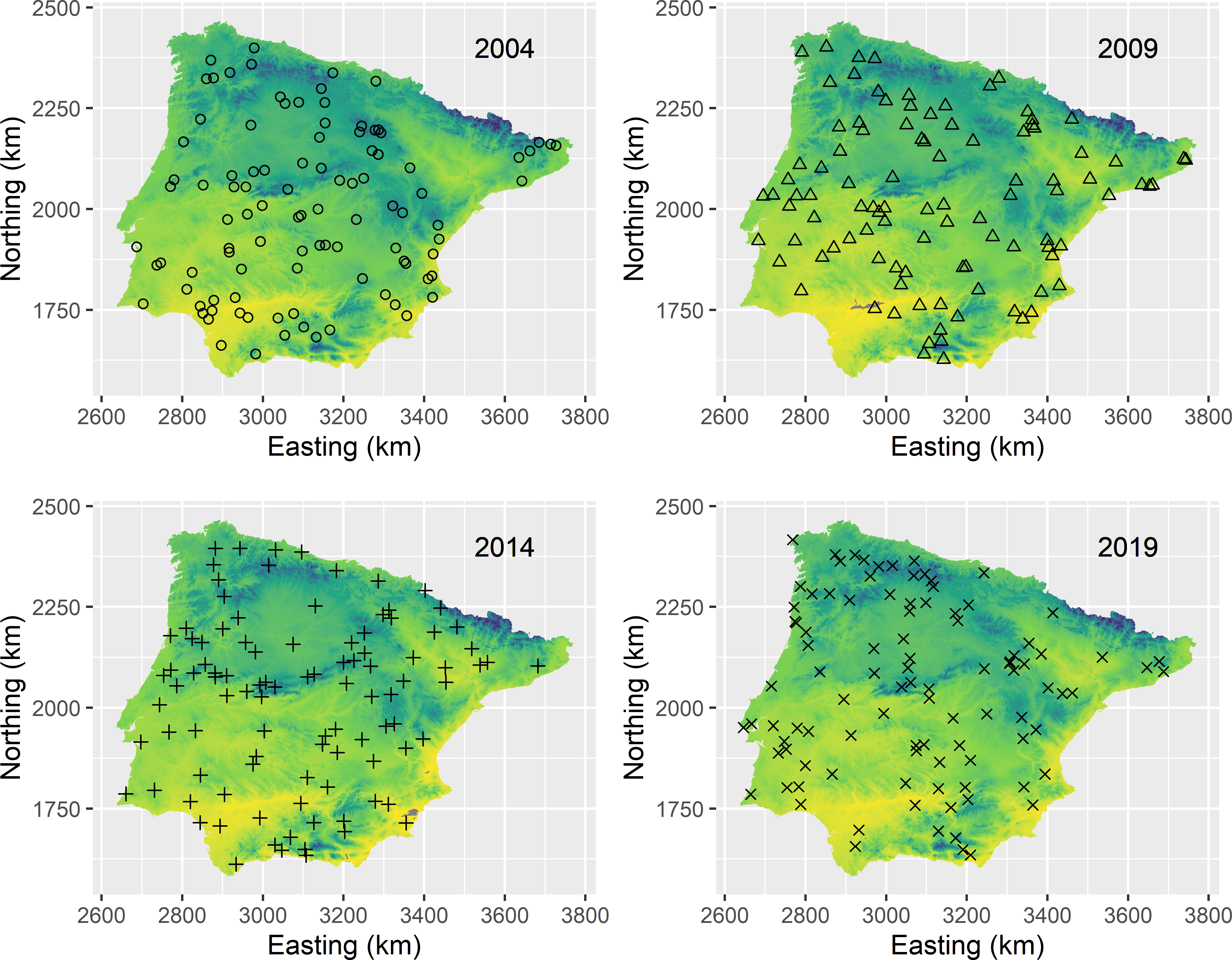
Figure 15.4: Independent synchronous space-time sample from Iberia. Locations are selected by simple random sampling.
The spatial means are estimated with the \(\pi\) estimator as there is no partial overlap of the spatial samples. All covariances of the mean estimators are zero. Estimation of the space-time parameters is done as before with the SS space-time sample. Four data frames of \(n\) rows are first made with the data observed in a specific panel. The variables of these four data frames are joined into a single data frame. The spatial means at the four times are then estimated by the sample means, computed with function apply.
panel_a <- filter(mysample_IS, panel == "a") %>% dplyr::select(TAS2004)
panel_b <- filter(mysample_IS, panel == "b") %>% dplyr::select(TAS2009)
panel_c <- filter(mysample_IS, panel == "c") %>% dplyr::select(TAS2014)
panel_d <- filter(mysample_IS, panel == "d") %>% dplyr::select(TAS2019)
panel_abcd <- cbind(panel_a, panel_b, panel_c, panel_d)
mz <- apply(panel_abcd, MARGIN = 2, FUN = mean)
C <- var(panel_abcd) / n
C[row(C) != col(C)] <- 0
#current mean
mz_cur_IS <- mz[4]
se_mz_cur_IS <- sqrt(C[4, 4])
#change of mean
w <- c(-1, 0, 0, 1)
d_mz_IS <- t(w) %*% mz
se_d_mz_IS <- sqrt(t(w) %*% C %*% w)
#trend of mean
w <- (t - mean(t)) / sum((t - mean(t))^2)
mz_trend_IS <- t(w) %*% mz
se_mz_trend_IS <- sqrt(t(w) %*% C %*% w)
#space-time mean
w <- rep(1 / 4, 4)
mz_st_IS <- t(w) %*% mz
se_mz_st_IS <- sqrt(t(w) %*% C %*% w)
15.4.3 Serially alternating design
To select an SA space-time sample with a period of two, \(2n=200\) sampling locations are selected. A variable is added to mysample_SA indicating the panel of the sampling locations. Figure 15.5 shows the selected SA space-time sample.
units <- sample(nrow(grd), size = 2 * n, replace = TRUE)
mysample_SA <- grd[units, ]
mysample_SA$panel <- rep(c("a", "b"), each = n)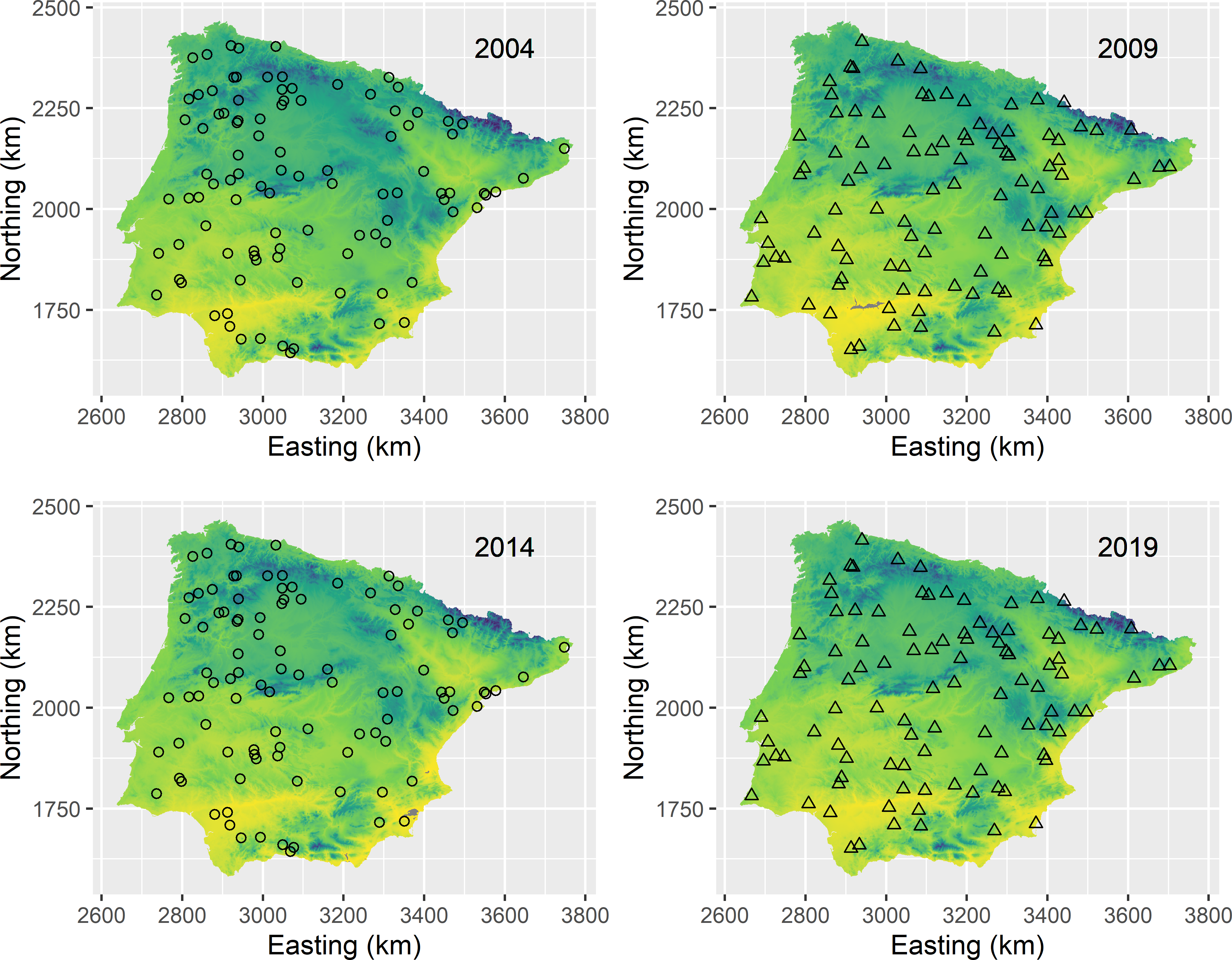
Figure 15.5: Serially alternating space-time sample from Iberia. Locations are selected by simple random sampling.
In SA sampling there is no partial overlap of the spatial samples at different times: there is either no coordinated overlap or full overlap. Spatial means therefore can be estimated by the usual \(\pi\) estimator. Two data frames of \(n\) rows are first made with the data observed in a specific panel. The variables of these two data frames are joined into a single data frame. The spatial means at the four times are then estimated by the sample means, computed with function apply.
panel_a <- filter(mysample_SA, panel == "a") %>% dplyr::select(TAS2004, TAS2014)
panel_b <- filter(mysample_SA, panel == "b") %>% dplyr::select(TAS2009, TAS2019)
panel_ab <- cbind(panel_a[1], panel_b[1], panel_a[2], panel_b[2])
mz <- apply(panel_ab, MARGIN = 2, FUN = mean)
To compute the matrix with estimated variances and covariances of the spatial mean estimators, first the full matrix is computed. Then the estimated covariances of spatial means of consecutive surveys are replaced by zeroes as the samples of these consecutive surveys are selected independently from each other, so that the two estimators are independent. Estimation of the space-time parameters is done as before with the SS space-time sample.
C <- var(panel_ab) / n
odd <- c(1, 3)
C[row(C) %in% odd & !(col(C) %in% odd)] <- 0
C[!(row(C) %in% odd) & col(C) %in% odd] <- 0
#current mean
mz_cur_SA <- mz[4]
se_mz_cur_SA <- sqrt(C[4, 4] / n)
#change of mean from time 1 to time 4
w <- c(-1, 0, 0, 1)
d_mz_SA <- t(w) %*% mz
se_d_mz_SA <- sqrt(t(w) %*% C %*% w)
#trend of mean
w <- (t - mean(t)) / sum((t - mean(t))^2)
mz_trend_SA <- t(w) %*% mz
se_mz_trend_SA <- sqrt(t(w) %*% C %*% w)
#space-time mean
mz_st_SA <- mean(mz)
w <- rep(1 / 4, 4)
se_mz_st_SA <- sqrt(t(w) %*% C %*% w)
15.4.4 Supplemented panel design
With SP sampling and four sampling times we have five panels: one panel with fixed sampling locations and four panels with swarming locations (Figure 15.1). Each panel consists of \(n/2\) sampling locations, so in total \(5n/2=250\) locations are selected. A variable indicating the panel is added to the data frame with the selected sampling locations. Figure 15.6 shows the selected SP sample.
units <- sample(nrow(grd), size = 5 * n / 2, replace = TRUE)
mysample_SP <- grd[units, ]
mysample_SP$panel <- rep(c("a", "b", "c", "d", "e"), each = n / 2)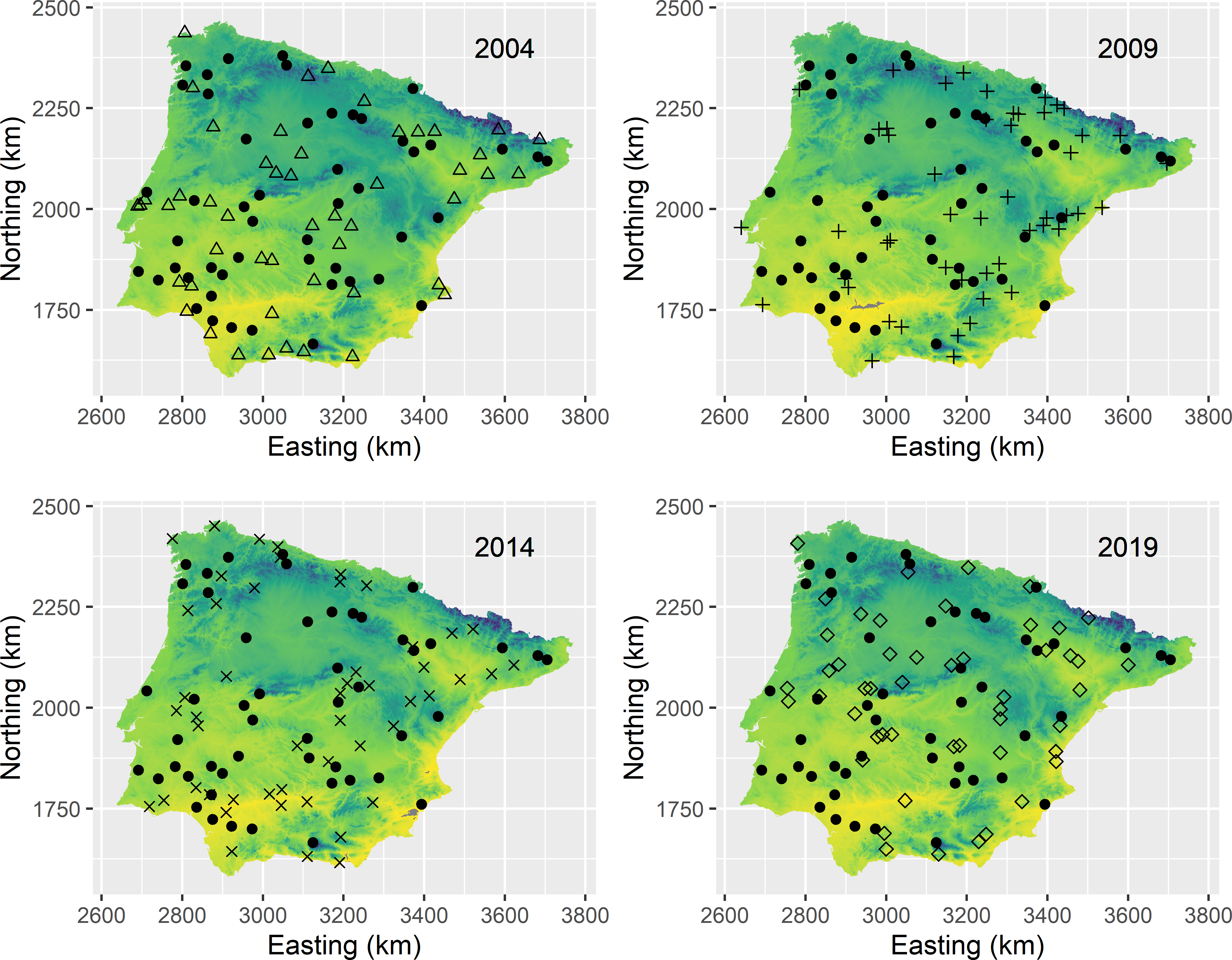
Figure 15.6: Supplemented panel space-time sample from Iberia. Locations are selected by simple random sampling. The permanent sampling locations are indicated by the filled dots, the swarming locations by the other symbols.
With SP sampling, the spatial means are estimated by the design-based GLS estimator (Equation (15.10)). As a first step, the eight elementary estimates (two per sampling time) are computed and collected in a vector. Note the order of the elementary estimates: first the estimated spatial means of 2004, 2009, 2014, and 2019, estimated from the panel with fixed sampling locations, then the spatial means estimated from the panels with swarming locations. The design matrix \(\mathbf{X}\) corresponding to this order of elementary estimates is constructed.
mz_1 <- tapply(
  mysample_SP$TAS2004, INDEX = mysample_SP$panel, FUN = mean)[c(1, 2)]
mz_2 <- tapply(
  mysample_SP$TAS2009, INDEX = mysample_SP$panel, FUN = mean)[c(1, 3)]
mz_3 <- tapply(
  mysample_SP$TAS2014, INDEX = mysample_SP$panel, FUN = mean)[c(1, 4)]
mz_4 <- tapply(
  mysample_SP$TAS2019, INDEX = mysample_SP$panel, FUN = mean)[c(1, 5)]
mz_el <- c(mz_1["a"], mz_2["a"], mz_3["a"], mz_4["a"],
           mz_1["b"], mz_2["c"], mz_3["d"], mz_4["e"])
X <- rbind(diag(4), diag(4))
The variances and covariances of the elementary estimates of the panel with fixed locations (SS subsample) are estimated, as well as the variances of the elementary estimates of the panels with swarming locations (IS subsample). The two variance-covariance matrices and a 4 \(\times\) 4 submatrix with all zeroes are combined into a single matrix, see matrix (15.11).
C_SS <- filter(mysample_SP, panel == "a") %>%
  dplyr::select(TAS2004, TAS2009, TAS2014, TAS2019) %>%
  var() / (n / 2)
C_IS <- cbind(mysample_SP$TAS2004[mysample_SP$panel == "b"],
              mysample_SP$TAS2009[mysample_SP$panel == "c"],
              mysample_SP$TAS2014[mysample_SP$panel == "d"],
              mysample_SP$TAS2019[mysample_SP$panel == "e"]) %>%
  var() / (n / 2)
C_IS[row(C_IS) != col(C_IS)] <- 0
zeroes <- matrix(0, nrow = 4, ncol = 4)
C <- rbind(cbind(C_SS, zeroes), cbind(zeroes, C_IS))
The design-based GLS estimates of the spatial means can be computed as follows, see Equation (15.10).
XCXinv <- solve(crossprod(X, solve(C, X)))
XCz <- crossprod(X, solve(C, mz_el))
mz_GLS <- XCXinv %*% XCz
Computing the estimated space-time parameters from the design-based GLS estimated spatial means is straightforward.
#current mean
mz_cur_SP <- mz_GLS[4]
se_mz_cur_SP <- sqrt(XCXinv[4, 4])
#change of mean
w <- c(-1, 0, 0, 1)
d_mz_SP <- t(w) %*% mz_GLS
se_d_mz_SP <- sqrt(t(w) %*% XCXinv %*% w)
#trend of mean
w <- (t - mean(t)) / sum((t - mean(t))^2)
mz_trend_SP <- t(w) %*% mz_GLS
se_mz_trend_SP <- sqrt(t(w) %*% XCXinv %*% w)
#space-time mean
w <- rep(1 / 4, 4)
mz_st_SP <- t(w) %*% mz_GLS
se_mz_st_SP <- sqrt(t(w) %*% XCXinv %*% w)
15.4.5 Rotating panel design
Similar to the SP design, with an in-for-two RP design and four sampling times we have five panels, each consisting of \(n/2\) sampling locations, so that in total \(5n/2=250\) locations are selected. Figure 15.7 shows the selected space-time sample.
units <- sample(nrow(grd), size = 5 * n / 2, replace = TRUE)
mysample_RP <- grd[units, ]
mysample_RP$panel <- rep(c("a", "b", "c", "d", "e"), each = n / 2)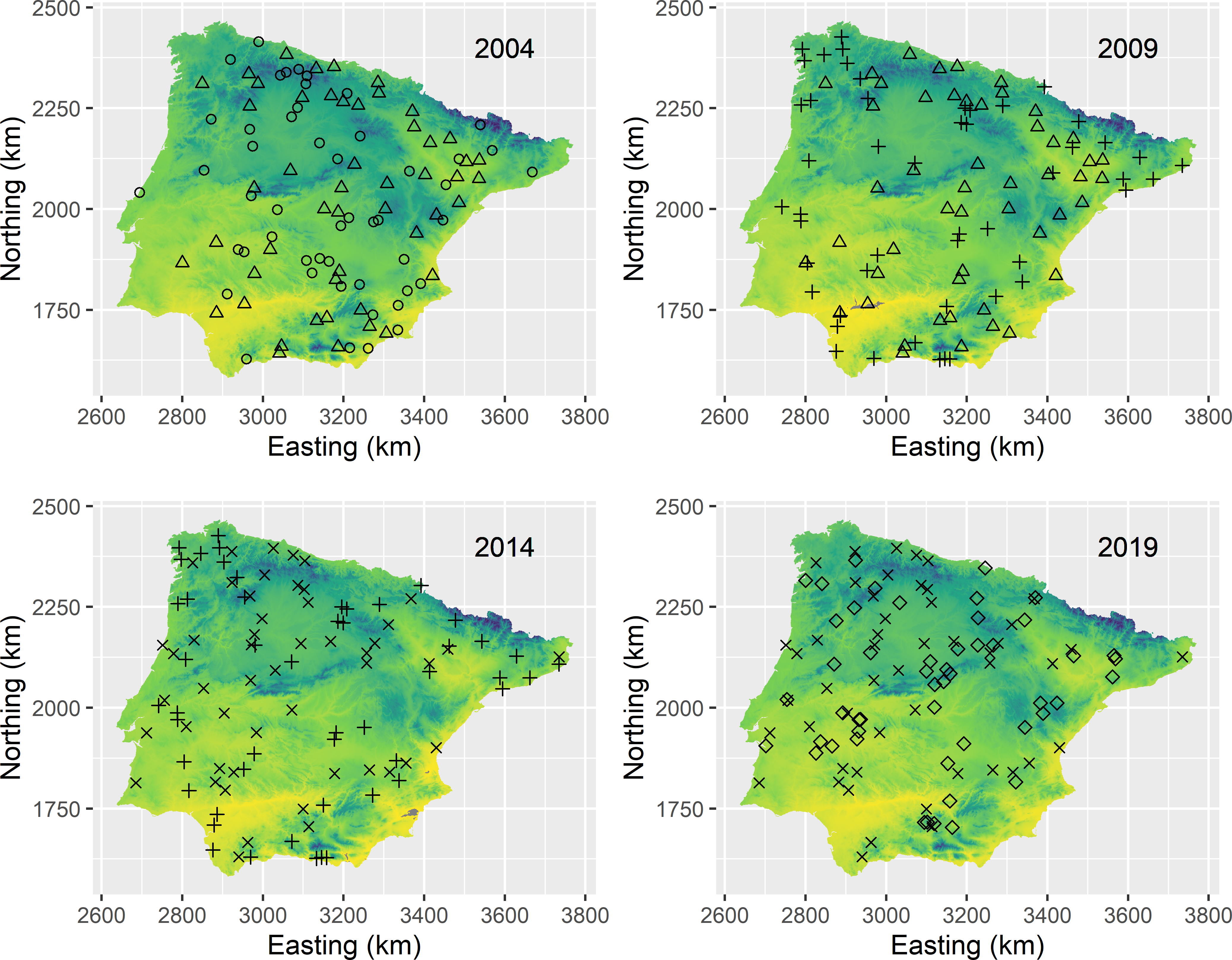
Figure 15.7: In-for-two rotating panel space-time sample from Iberia. Locations are selected by simple random sampling. Half of the sampling locations observed in a given year are also observed in the consecutive survey.
Two elementary estimates per sampling time are computed and collected in a vector. Note that now the elementary estimates are ordered by sampling time. The design matrix corresponding to this order is constructed.
mz_1 <- tapply(
  mysample_RP$TAS2004, INDEX = mysample_RP$panel, FUN = mean)[c(1, 2)]
mz_2 <- tapply(
  mysample_RP$TAS2009, INDEX = mysample_RP$panel, FUN = mean)[c(2, 3)]
mz_3 <- tapply(
  mysample_RP$TAS2014, INDEX = mysample_RP$panel, FUN = mean)[c(3, 4)]
mz_4 <- tapply(
  mysample_RP$TAS2019, INDEX = mysample_RP$panel, FUN = mean)[c(4, 5)]
mz_el <- c(mz_1, mz_2, mz_3, mz_4)
X <- matrix(c(rep(c(1, 0, 0, 0), 2),
              rep(c(0, 1, 0, 0), 2),
              rep(c(0, 0, 1, 0), 2),
              rep(c(0, 0, 0, 1), 2)), nrow = 8, ncol = 4, byrow = TRUE)
To construct the variance-covariance matrix of the eight elementary estimates, first the 2 \(\times\) 2 matrices with estimated variances and covariances are computed for panels b, c, and d. These three panels are used to estimate the spatial means of two consecutive years: the locations of panel b are used to estimate the spatial means for 2004 and 2009, panel c for 2009 and 2014, and panel d for 2014 and 2019 (Figure 15.1). These three matrices are copied into the 8 \(\times\) 8 matrix, see matrix (15.12). Finally, the data of panel a and e are used to compute the estimated variances of the estimators of the spatial means in 2004 and 2019, respectively, and copied to the upper left and lower right entry of the variance-covariance matrix, respectively.
C_b <- filter(mysample_RP, panel == "b") %>% dplyr::select(TAS2004, TAS2009) %>%
  var() / (n / 2)
C_c <- filter(mysample_RP, panel == "c") %>% dplyr::select(TAS2009, TAS2014) %>%
  var() / (n / 2)
C_d <- filter(mysample_RP, panel == "d") %>% dplyr::select(TAS2014, TAS2019) %>%
  var() / (n / 2)
C <- matrix(data = 0, ncol = 8, nrow = 8)
C[2:3, 2:3] <- C_b
C[4:5, 4:5] <- C_c
C[6:7, 6:7] <- C_d
C[1, 1] <- var(mysample_RP[mysample_RP$panel == "a", "TAS2004"]) / (n / 2)
C[8, 8] <- var(mysample_RP[mysample_RP$panel == "e", "TAS2019"]) / (n / 2)
The design-based GLS estimates of the spatial means for the four sampling times are computed as before, followed by computing the estimated space-time parameters.
XCXinv <- solve(crossprod(X, solve(C, X)))
XCz <- crossprod(X, solve(C, mz_el))
mz_GLS <- XCXinv %*% XCz
#current mean
mz_cur_RP <- mz_GLS[4]
se_mz_cur_RP <- sqrt(XCXinv[4, 4])
#change of mean
w <- c(-1, 0, 0, 1)
d_mz_RP <- t(w) %*% mz_GLS
se_d_mz_RP <- sqrt(t(w) %*% XCXinv %*% w)
#trend of mean
w <- (t - mean(t)) / sum((t - mean(t))^2)
mz_trend_RP <- t(w) %*% mz_GLS
se_mz_trend_RP <- sqrt(t(w) %*% XCXinv %*% w)
#space-time mean
w <- rep(1 / 4, 4)
mz_st_RP <- t(w) %*% mz_GLS
se_mz_st_RP <- sqrt(t(w) %*% XCXinv %*% w)
15.4.6 Sampling experiment
The random sampling with the five space-time designs and estimation of the four space-time parameters is repeated 10,000 times. The standard deviations of the 10,000 estimates of a space-time parameter are shown in Table 15.1. Note that to determine the standard errors of the estimators of the space-time parameters for the SS, IS, and SA designs, a sampling experiment is not really needed. These can be computed without error because we have exhaustive knowledge of the study variable at all sampling times. However, for the SP and RP designs, a sampling experiment is needed to approximate the design-expectation of the standard error of the estimators of the space-time parameters. This is because the space-time parameters are derived from the GLS estimator of the spatial means, and the GLS estimator is a function of the estimated covariances of the elementary estimates (Equation (15.10)). Using the true covariance of the elementary estimates in the GLS estimator, instead of the estimated covariance, leads to an underestimation of the standard error. Computing the true standard errors of the estimators of the space-time parameters for the various space-time designs is left as an exercise.
As a reference for the standard deviations in Table 15.1: the current mean (spatial mean air temperature in 2019) equals 14.59\(^\circ\)C, the change of the mean from 2004 to 2019 equals 0.611\(^\circ\)C, the temporal trend equals 0.198\(^\circ\)C per five years, and the space-time mean equals 14.44\(^\circ\)C.
| Current mean | Change of mean | Trend of mean | Space-time mean | |
|---|---|---|---|---|
| SS | 0.2709 | 0.0343 | 0.0123 | 0.2741 |
| IS | 0.2653 | 0.3873 | 0.1221 | 0.1354 |
| SA | 0.2676 | 0.3894 | 0.0787 | 0.1910 |
| SP | 0.1755 | 0.0481 | 0.0171 | 0.1770 |
| RP | 0.1769 | 0.0840 | 0.0299 | 0.1744 |
Estimates of the current mean with the SP and RP designs are much more precise than with the SS, IS, and SA designs. This is because with designs SP and RP there is partial overlap with the samples of the other years. If the study variable at different years is correlated, we can profit from the data of previous years. In our case, this correlation is very strong:
          TAS2004   TAS2009   TAS2014   TAS2019
TAS2004 1.0000000 0.9950227 0.9878301 0.9927014
TAS2009 0.9950227 1.0000000 0.9875005 0.9960541
TAS2014 0.9878301 0.9875005 1.0000000 0.9938060
TAS2019 0.9927014 0.9960541 0.9938060 1.0000000
The differences in standard deviations of the estimated current means among the SS, IS, and SA designs are due to random variation: the true standard errors of the current mean estimator are equal for these three space-time designs.
The strong correlation also explains that the estimated change of the spatial mean from 2004 to 2019 with the SS design is much more precise than with the IS and SA designs. With the IS and SA designs, the sample of 2019 is selected independently from the sample of 2004, so that the covariance of the two spatial mean estimators is zero. With the SS design this covariance is subtracted two times from the sum of the variances of the spatial mean estimators. The standard error of the estimator of the change of the spatial mean from 2009 to 2019 with the SA design (not shown in Table 15.1) is much smaller than that of the change from 2004 to 2019, because the spatial means at these two times are estimated from the same sample, so that we profit from the strong positive correlation. The standard error of the change estimator with the SP design is slightly larger than the standard error with the SS design, because with this design there is only partial overlap, so that we profit less from the correlation. The standard error with the RP design is larger than that of the SP design, because with the RP design there is no overlap of the samples of 2004 and 2019 (Figure 15.1). Despite the absence of overlap, the standard error is still considerably smaller than those with the IS and SA designs because the spatial means of 2004 and 2019 are estimated by the GLS estimator that uses the data of all years, so that we still profit from the correlation.
Estimation of the temporal trend of the spatial mean is most precise with the SS design, closely followed by the SP design, and least precise with the IS design. This is in agreement with the results of Brus and de Gruijter (2011) and Brus and de Gruijter (2013). On the contrary, estimation of the space-time mean is most precise with the IS design and least precise with the SS design. With strong persistence of the spatial patterns, as in our case, it is not efficient to observe the same sampling locations at all times when interest is in the space-time mean. In our case with very strong correlation, the larger the total number of sampling locations over all sampling times, the smaller the standard error of the space-time mean estimator. The total number of sampling locations in this case study are \(n\) with SS, \(4n\) with IS, \(2n\) with SA, and \(5n/2\) with SP and RP.
15.5 Space-time sampling with stratified random sampling in space
In real-world applications, one will often use more efficient sampling designs than simple random sampling for selecting spatial sampling units. For instance, in the case study of the previous section, stratified simple random sampling using climate zones is most likely more efficient than simple random sampling.
To select a space-time sample with stratified simple random sampling as a spatial design, the selection procedures described above for the five basic types of space-time design are applied at the level of the strata. Estimation of the space-time parameters goes along the same lines, using the \(\pi\) estimator of the spatial mean and the estimator of the standard error presented in Chapter 4. With the SP and RP designs, the covariance of the elementary estimators of the spatial means at two sampling times using the data of the same panel, can be estimated by
\[\begin{equation} \widehat{C}_{ab} = \sum_{h=1}^H w^2_h \frac{\widehat{S^2}_{abh}}{m_h} \;, \tag{15.19} \end{equation}\]
with \(\widehat{S^2}_{abh}\) the estimated covariance of the study variable at times \(t_a\) and \(t_b\) in stratum \(h\), and \(m_h\) the number of sampling locations in the panel in stratum \(h\).
Interesting new developments are presented by Z. Wang and Zhu (2019) and Zhao and Grafström (2020).
Exercises
- Compute for the annual mean temperature data of Iberia the true standard error of the estimator of (i) the spatial mean in 2019; (ii) the change of the spatial mean from 2004 to 2019; (iii) the temporal trend of the spatial mean (average change per five years in the period from 2004 to 2019); and (iv) the space-time mean, for all five space-time designs and simple random sampling with replacement of 100 units per time. Use for the designs SP and RP the true covariances of the elementary estimates in the GLS estimators of the spatial means.
- With an SP and an RP design, the change of the mean can also be estimated by the difference of the \(\pi\) estimates of the spatial means at the two times, instead of the difference of the two GLS estimates. The variance of the difference of the \(\pi\) estimators of two simple random samples at different times with partial overlap equals \[\begin{equation} V(\bar{d}_{ab})=\frac{S^2_a}{n} + \frac{S^2_b}{n} - 2\frac{m\;S^2_{ab}}{n^2}\;, \tag{15.20} \end{equation}\] with \(S^2_a\) and \(S^2_b\) the spatial variance at time \(t_a\) and \(t_b\), respectively, \(S^2_{ab}\) the spatial covariance of the study variable at times \(t_a\) and \(t_b\), \(n\) the size of the simple random samples, and \(m\) the number of units observed at both times. Compute for Iberia the standard error of the estimator of the change of the mean with Equation (15.20), using the true spatial variances and covariances for 2004 and 2019, for simple random samples of size 100 (\(n=100\)) and a matching proportion of 0.5 (\(m=50\)). Compare with the true standard error of the estimator of the change of the mean using the GLS estimators computed in the previous exercise. Explain that the standard error of the \(\pi\) estimators is larger than the standard error with the GLS estimators.