Chapter 19 Conditioned Latin hypercube sampling
This chapter and Chapter 20 on response surface sampling are about experimental designs that have been adapted for spatial surveys. Adaptation is necessary because, in contrast to experiments, in observational studies one is not free to choose any possible combination of levels of different factors. When two covariates are strongly positively correlated, it may happen that there are no population units with a relatively large value for one covariate and a relatively small value for the other covariate. By contrast, in experimental research it is possible to select any combination of factor levels.
In a full factorial design, all combinations of factor levels are observed. With \(k\) factors and \(l\) levels per factor, the total number of observations is \(l^k\). With numerous factors and/or numerous levels per factor, observing \(l^k\) experimental units becomes unfeasible in practice. Alternative experimental designs have been developed that need fewer observations but still provide detailed information about how the study variable responds to changes in the factor levels. This chapter will describe and illustrate the survey sampling analogue of Latin hypercube sampling. Response surface sampling follows in the next chapter.
Latin hypercube sampling is used in designing industrial processes, agricultural experiments, and computer experiments, with numerous covariates and/or factors of which we want to study the effect on the output (McKay, Beckman, and Conover 1979). A much cheaper alternative to a full factorial design is an experiment with, for all covariates, exactly one observation per level. So, in the agricultural experiment described in Chapter 16 with the application rates of N and P as factors and four levels for each factor, this would entail four observations only, distributed in a square in such way that we have in all rows and in all columns one observation, see Figure 19.1. This is referred to as a Latin square. The generalisation of a Latin square to a higher number of dimensions is a Latin hypercube (LH).
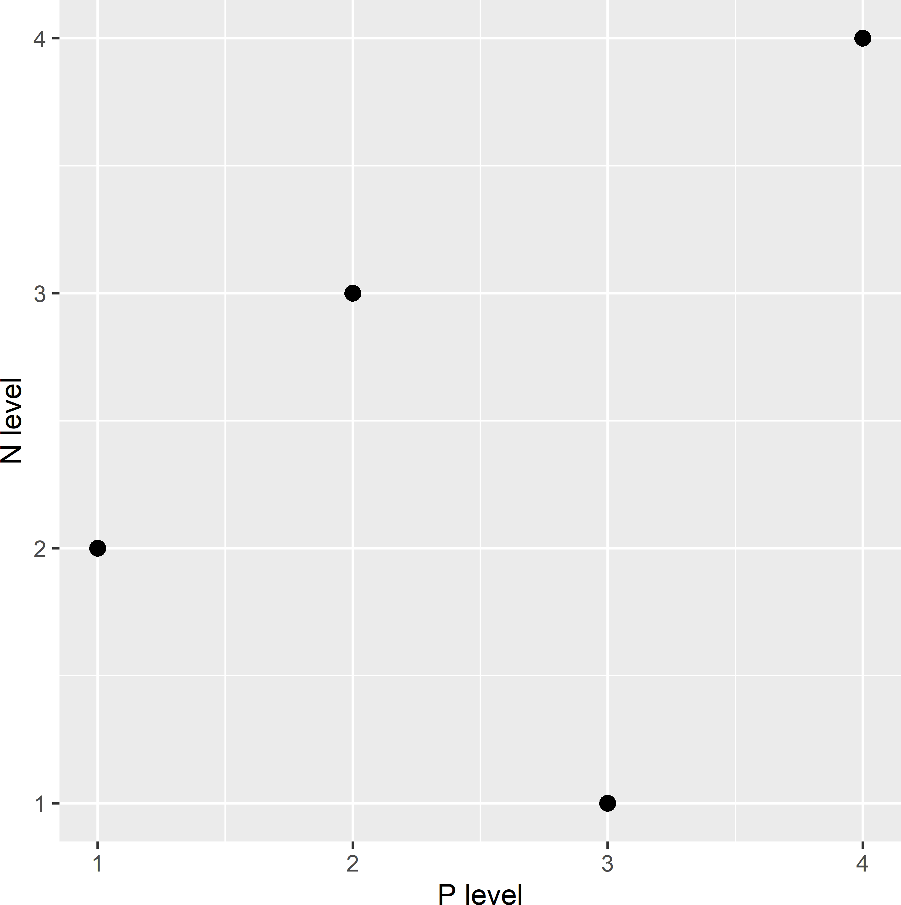
Figure 19.1: Latin square for agricultural experiment with four application rates of N and P.
Minasny and McBratney (2006) adapted LH sampling for observational studies; this adaptation is referred to as conditioned Latin hypercube (cLH) sampling. For each covariate, a series of intervals (marginal strata) is defined. The number of marginal strata per covariate is equal to the sample size, so that the total number of marginal strata equals \(p^n\), with \(p\) the number of covariates and \(n\) the sample size. The bounds of the marginal strata are chosen such that the numbers of raster cells in these marginal strata are equal. This is achieved by using the quantiles corresponding to evenly spaced cumulative probabilities as stratum bounds. For instance, for five marginal strata we use the quantiles corresponding to the cumulative probabilities 0.2, 0.4, 0.6, and 0.8.
The minimisation criterion proposed by Minasny and McBratney (2006) is a weighted sum of three components:
- O1: the sum over all marginal strata of the absolute deviations of the marginal stratum sample size from the targeted sample size (equal to 1);
- O2: the sum over all classes of categorical covariates of the absolute deviations of the sample proportion of a given class from the population proportion of that class; and
- O3: the sum over all entries of the correlation matrix of the absolute deviation of the correlation in the sample from the correlation in the population.
With cLH sampling, the marginal distributions of the covariates in the sample are close to these distributions in the population. This can be advantageous for mapping methods that do not rely on linear relations, for instance in machine learning techniques like classification and regression trees (CART), and random forests (RF). In addition, criterion O3 ensures that the correlations between predictors are respected in the sample set.
cLH samples can be selected with function clhs of package clhs (Roudier 2021). With this package, the criterion is minimised by simulated annealing, see Section 23.1 for an explanation of this optimisation method. Arguments iter, temp, tdecrease, and length.cycle of function clhs are control parameters of the simulated annealing algorithm. In the next code chunk, I use default values for these arguments. With argument weights, the weights of the components of the minimisation criterion can be set. The default weights are equal to 1.
Argument cost is for cost-constrained cLH sampling (Roudier, Hewitt, and Beaudette 2012), and argument eta can be used to control the sampling intensities of the marginal strata (Minasny and McBratney 2010). This argument is of interest if we would like to oversample the marginal strata near the edge of the multivariate distribution.
cLH sampling is illustrated with the five covariates of Eastern Amazonia that were used before in covariate space coverage sampling (Chapter 18).
library(clhs)
covs <- c("SWIR2", "Terra_PP", "Prec_dm", "Elevation", "Clay")
set.seed(314)
res <- clhs(
  grdAmazonia[, covs], size = 20, iter = 50000, temp = 1, tdecrease = 0.95,
  length.cycle = 10, progress = FALSE, simple = FALSE)
mysample_CLH <- grdAmazonia[res$index_samples, ]
Figure 19.2 shows the selected sample in a map of SWIR2. In Figure 19.3 the sample is plotted in a biplot of Prec_dm against SWIR2. Each black dot in the biplot represents one grid cell in the population. The vertical and horizontal lines in the biplot are at the bounds of the marginal strata of SWIR2 and Prec_dm, respectively. The number of grid cells between two consecutive vertical lines is constant, as well as the number of grid cells between two consecutive horizontal lines, i.e., the marginal strata have equal sizes. The intervals are the narrowest where the density of grid cells in the plot is highest. Ideally, in each column and row, there is exactly one sampling unit (red dot).
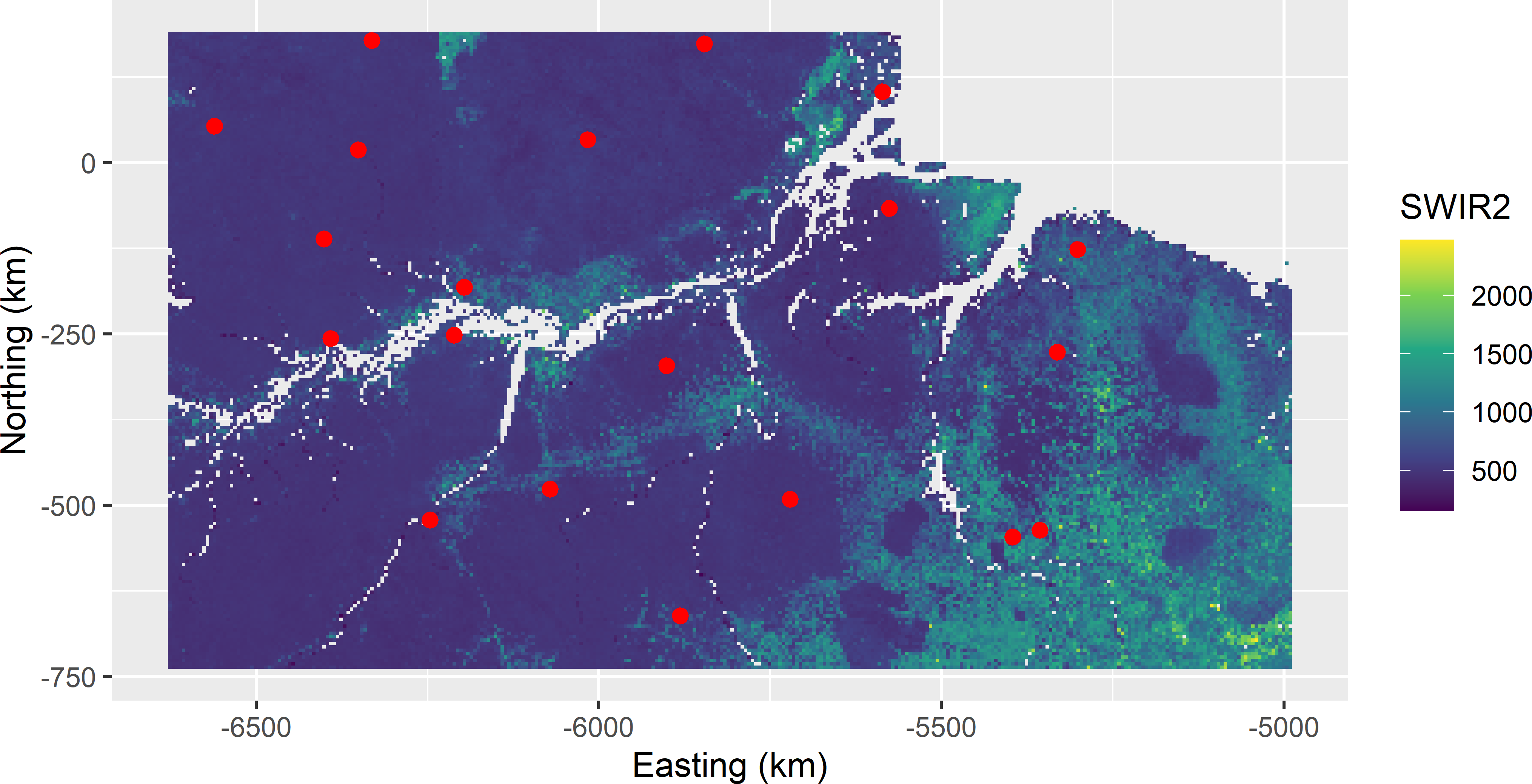
Figure 19.2: Conditioned Latin hypercube sample from Eastern Amazonia in a map of SWIR2.
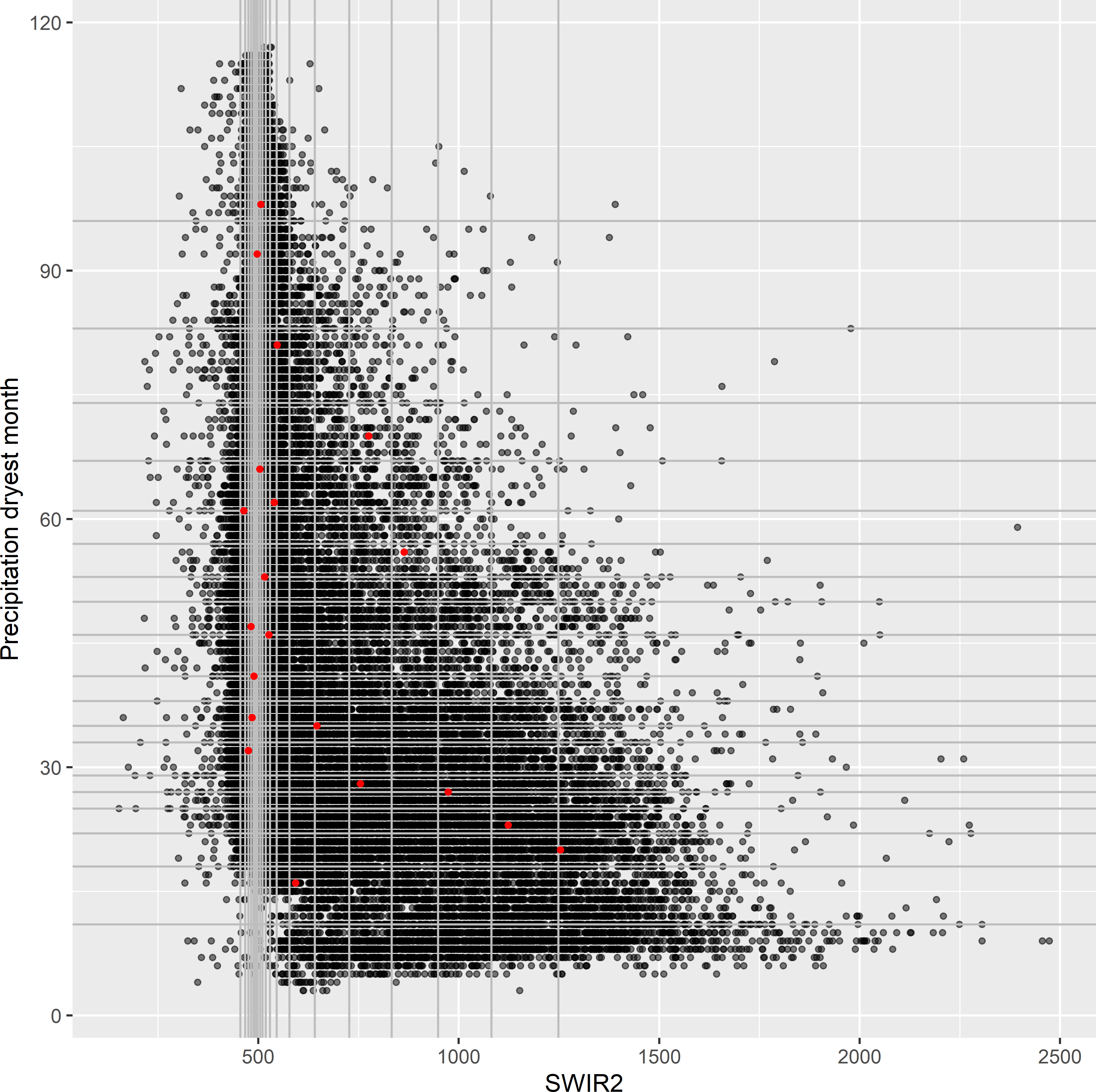
Figure 19.3: Conditioned Latin hypercube sample plotted in a biplot of precipitation in the dryest month against SWIR2. The vertical and horizontal lines are at the bounds of the marginal strata of the covariates SWIR2 and precipitation dryest month, respectively.
Figure 19.4 shows the sample sizes for all 100 marginal strata. The next code chunk shows how the marginal stratum sample sizes are computed.
probs <- seq(from = 0, to = 1, length.out = nrow(mysample_CLH) + 1)
bounds <- apply(grdAmazonia[, covs], MARGIN = 2,
  FUN = function(x) quantile(x, probs = probs))
mysample_CLH <- as.data.frame(mysample_CLH)
counts <- lapply(1:5, function(i)
  hist(mysample_CLH[, i + 3], bounds[, i], plot = FALSE)$counts)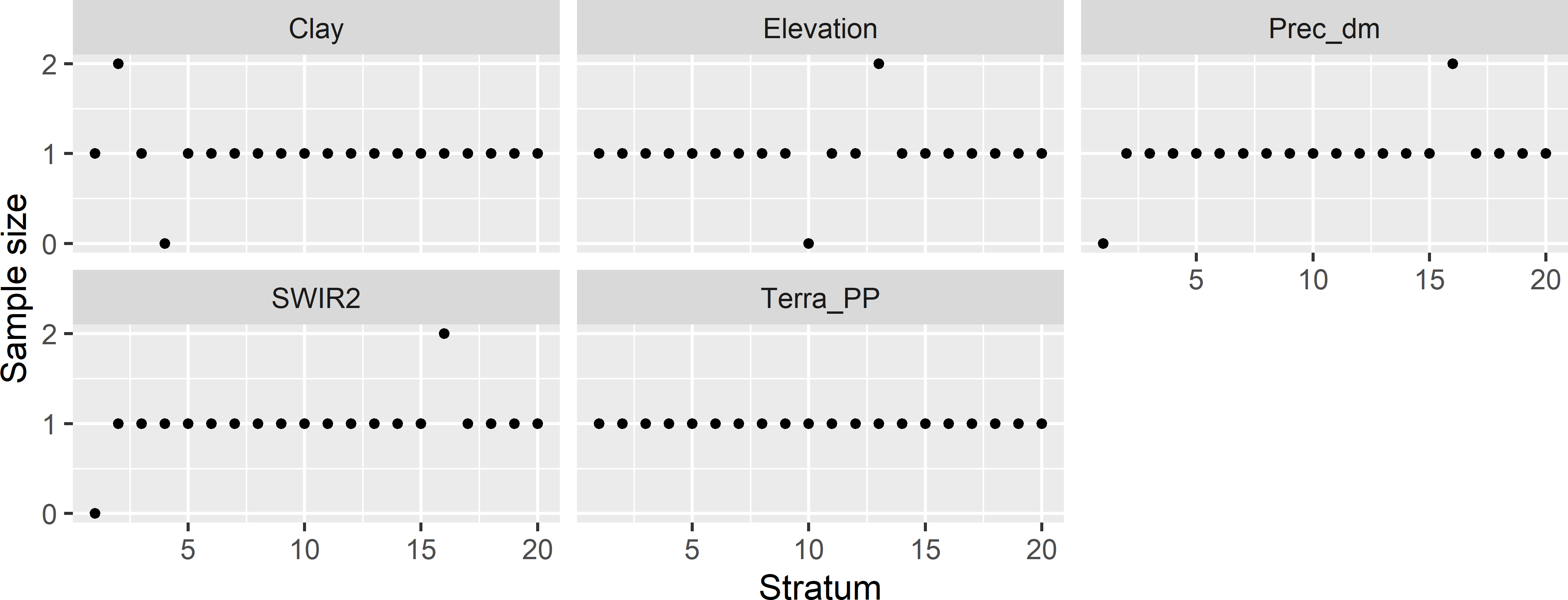
Figure 19.4: Sample sizes of marginal strata for the conditioned Latin hypercube sample of size 20 from Eastern Amazonia.
For all marginal strata with one sampling unit, the contribution to component O1 of the minimisation criterion is 0. For marginal strata with zero or two sampling units, the contribution is 1, for marginal strata with three sampling units the contribution equals 2, etc. In Figure 19.4 there are four marginal strata with zero units and four marginal strata with two units. Component O1 therefore equals 8 in this case.
Figure 19.5 shows the trace of the objective function, i.e., the values of the minimisation criterion during the optimisation. The trace plot indicates that 50,000 iterations are sufficient. I do not expect that the criterion can be reduced anymore. The final value of the minimisation criterion is extracted with function tail using argument n = 1.
[1] 9.51994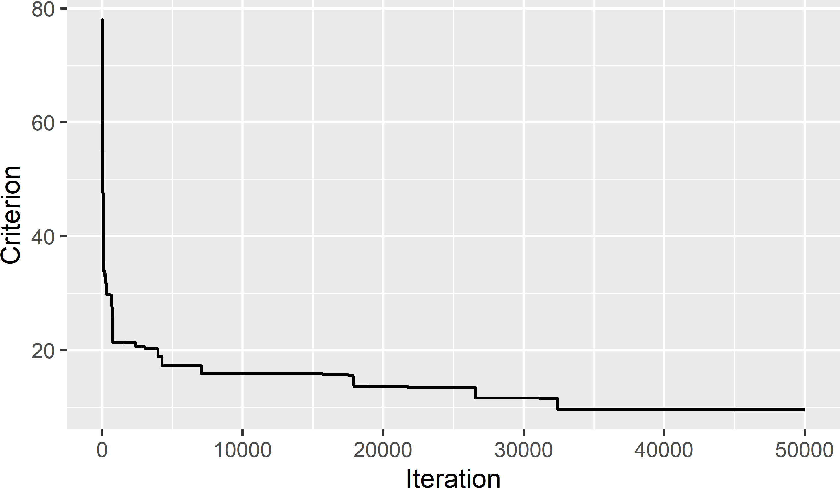
Figure 19.5: Trace of minimisation criterion during optimisation of conditioned Latin hypercube sampling from Eastern Amazonia.
In the next code chunk, the minimised value of the criterion is computed “by hand”.
countslf <- data.frame(counts = unlist(counts))
O1 <- sum(abs(countslf$counts - 1))
rho <- cor(grdAmazonia[, covs])
r <- cor(mysample_CLH[, covs])
O3 <- sum(abs(rho - r))
print(O1 + O3)
[1] 9.51994Exercises
- Use the data of Hunter Valley (
grdHunterValleyof package sswr) to select a cLH sample of size 50, using elevation_m, slope_deg, cos_aspect, cti, and ndvi as covariates. Plot the selected sample in a map of covariate cti, and plot the selected sample in a biplot of cti against elevation_m. In which part of the biplot are most units selected, and which part is undersampled?
- Load the simulated data of Figure 16.1 (
results/SimulatedSquare.rda), and select a cLH sample of size 16, using the covariate \(x\) and the spatial coordinates as stratification variables. Plot the selected sample in the square with simulated covariate values.- What do you think of the geographical spreading of the sampling units? Is it optimal?
- Compute the number of sampling units in the marginal strata of \(s1\), \(s2\), and the covariate \(x\). First, compute the bounds of these marginal strata. Are all marginal strata of \(s1\) and \(s2\) sampled? Suppose that all marginal strata of \(s1\) and \(s2\) are sampled (contain one sampling point), does this guarantee good spatial coverage?
- Plot the trace of the minimisation criterion, and retrieve the minimised value. Is this minimised value in agreement with the marginal stratum sample sizes?
19.1 Conditioned Latin hypercube infill sampling
Package clhs can also be used for selecting a conditioned Latin hypercube sample in addition to existing sampling units (legacy sample), as in spatial infill sampling (Section 17.2). The units of the legacy sample are assigned to argument must.include. Argument size must be set to the total sample size, i.e., the number of mandatory units (legacy sample units) plus the number of additional infill units.
To illustrate conditioned Latin hypercube infill sampling (cLHIS), in the next code chunk I select a simple random sample of ten units from Eastern Amazonia to serve as the legacy sample. Twenty new units are selected by cLHIS. The ten mandatory units (i.e., units which are already sampled and thus must be in the sample set computed by cLHIS) are at the end of the vector with the index of the selected raster cells.
set.seed(314)
units <- sample(nrow(grdAmazonia), 10, replace = FALSE)
res <- clhs(grdAmazonia[, covs], size = 30, must.include = units,
  tdecrease = 0.95, iter = 50000, progress = FALSE, simple = FALSE)
mysample_CLHI <- grdAmazonia[res$index_samples, ]
mysample_CLHI$free <- as.factor(rep(c(1, 0), c(20, 10)))
Figure 19.6 shows the selected cLHI sample in a map of SWIR2. In Figure 19.7 the sample is plotted in a biplot of SWIR2 against Prec_dm. The marginal strata already covered by the legacy sample are mostly avoided by the additional sample.
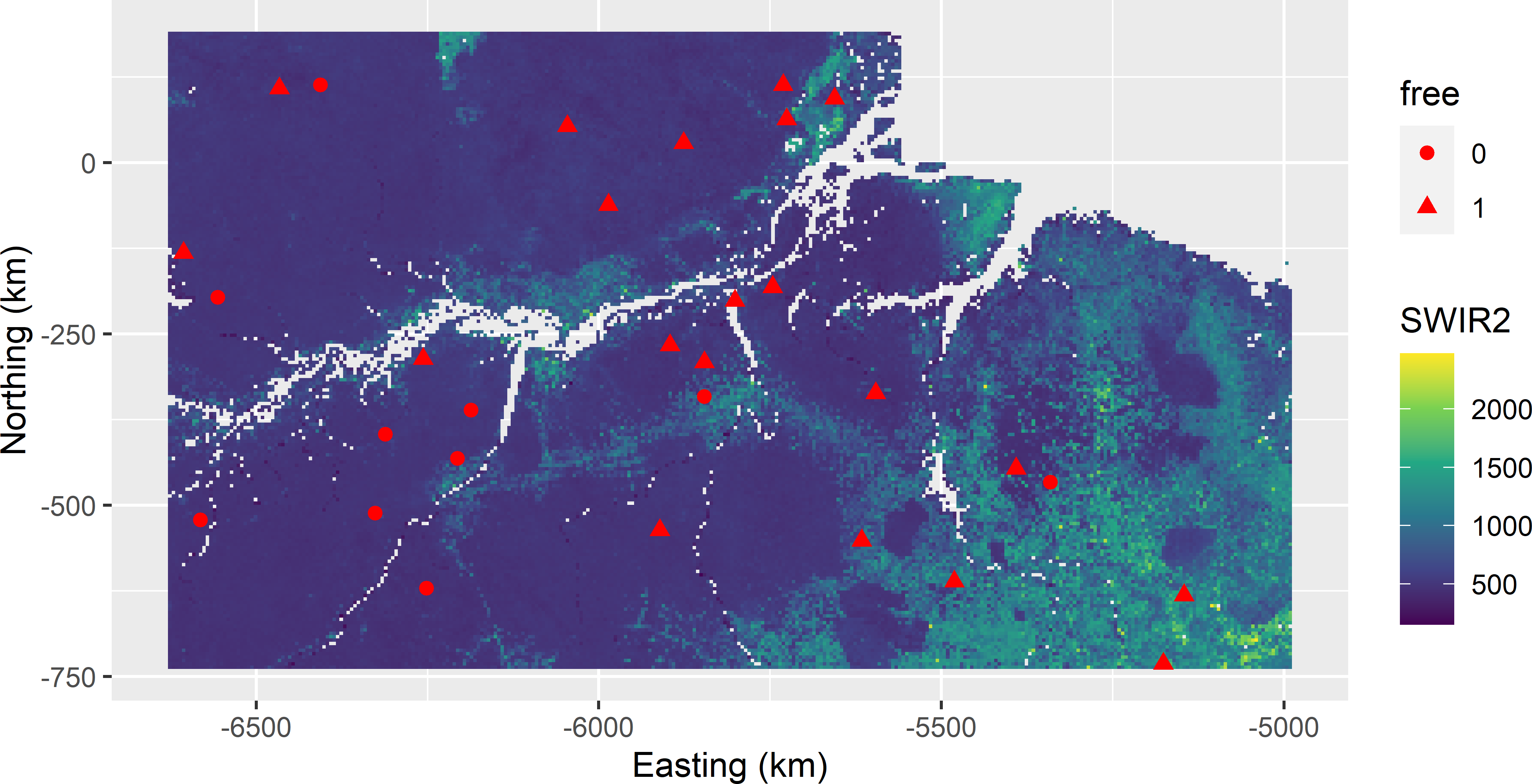
Figure 19.6: Conditioned Latin hypercube infill sample from Eastern Amazonia in a map of SWIR2. Legacy units have free-value 0; infill units have free-value 1.
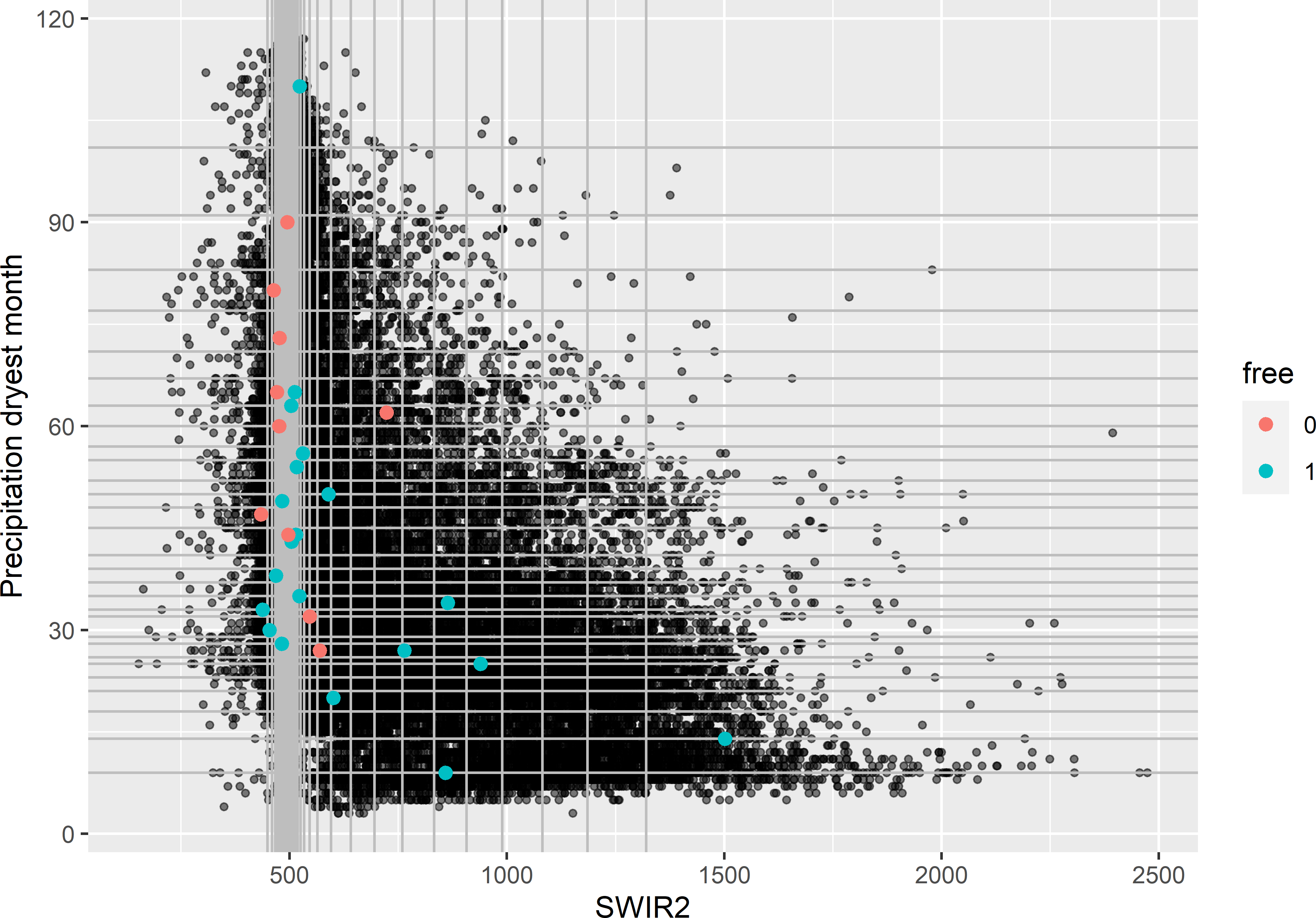
Figure 19.7: Conditioned Latin hypercube infill sample plotted in a biplot of SWIR2 against precipitation in the dryest month. Legacy units have free-value 0; infill units have free-value 1.
19.2 Performance of conditioned Latin hypercube sampling in random forest prediction
The performance of cLH sampling is studied in the same experiment as covariate space coverage sampling of the previous chapter. In total, 500 cLH samples of size 25 are selected and an equal number of samples of sizes 50 and 100. Each sample is used to calibrate a RF model for the aboveground biomass (AGB) using five covariates as predictors. The calibrated models are used to predict AGB at the 25,000 validation units selected by simple random sampling without replacement. Simple random (SI) sampling is added as a reference sampling design that ignores the covariates. The prediction errors are used to estimate three map quality indices, the population mean error (ME), the population root mean squared error (RMSE), and the population Nash-Sutcliffe model efficiency coefficient (MEC), see Chapter 25.
Figure 19.8 shows the results as boxplots, each based on 500 estimates. For \(n=25\) and \(100\), cLH sampling performs best in terms of RMSE and MEC, whereas for \(n=50\) CSC sampling performs best. For \(n=25\) and \(50\), the boxplots of cLH and SI show quite a few outliers with large values of RMSE, resulting in small values of MEC. For CSC, these map quality indices are more stable. Remarkably, for \(n=100\) SI sampling performs about equally to CSC and cLH sampling.
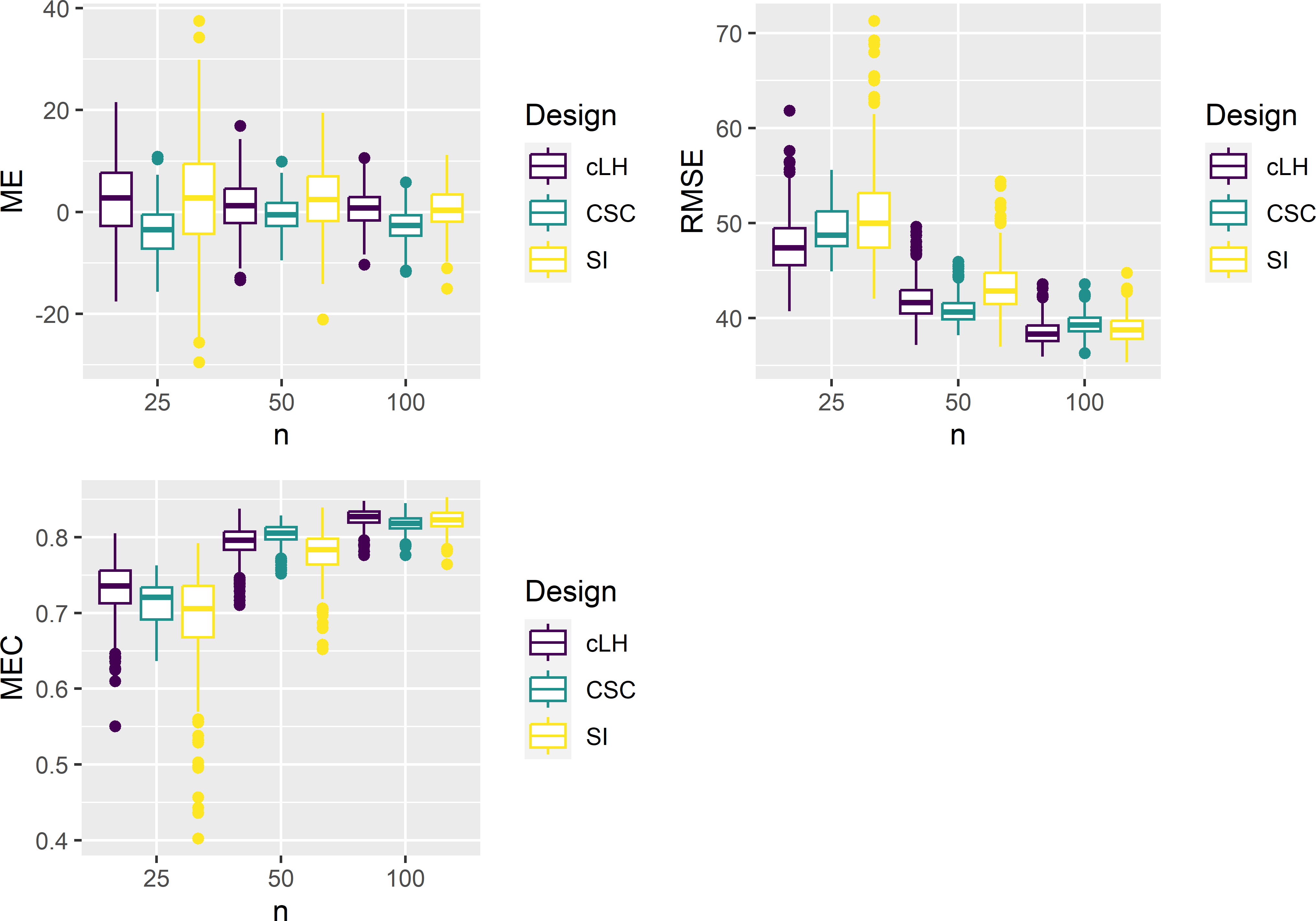
Figure 19.8: Boxplots of ME, RMSE, and MEC of predictions with RF models calibrated on conditioned Latin hypercube (cLH), covariate space coverage (CSC), and simple random (SI) samples from Eastern Amazonia, for sample sizes of 25, 50, and 100 units.
In Figure 19.9 the RMSE is plotted against the minimised criterion (O1 + O3) for the cLH and the SI samples. For all three sample sizes, there is a weak positive correlation of the minimisation criterion and the RMSE: for \(n=25\), 50, and 100 this correlation is 0.369, 0.290, and 0.140, respectively. On average, cLH performs slightly better than SI for \(n=25\) (Table 19.1). The gain in accuracy decreases with the sample size. For \(n=100\), the two designs perform about equally. Especially for \(n=25\) and 50, the distribution of RMSE with SI has a long right tail. For these small sample sizes, the risk of selecting an SI sample leading to a poor map with large RMSE is much larger than with cLH sampling.
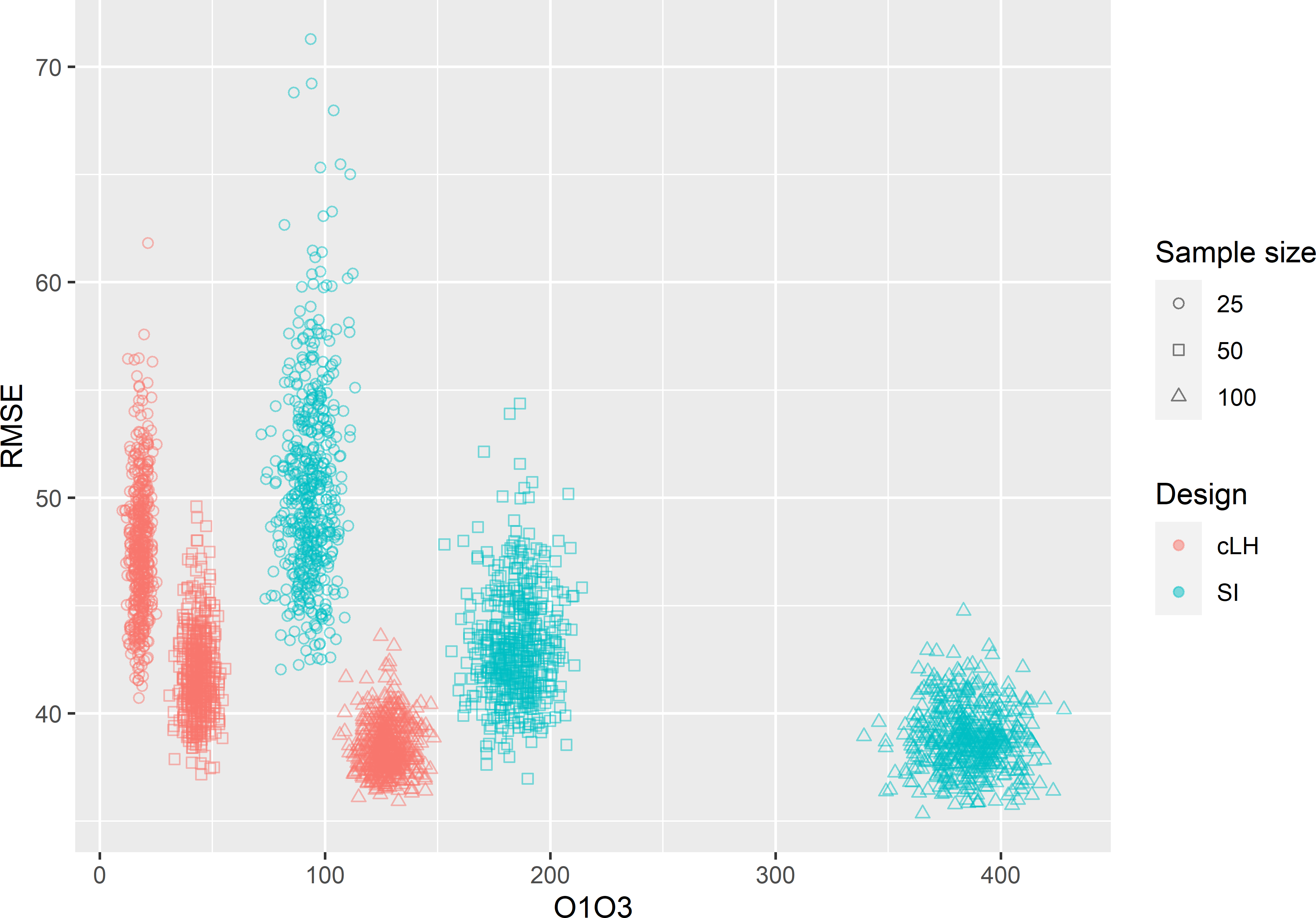
Figure 19.9: Biplot of the minimisation criterion (O1 + O3) and the RMSE of RF predictions of AGB in Eastern Amazonia for conditioned Latin hypercube (cLH) sampling and simple random (SI) sampling, and three sample sizes.
| Sample size | cLH | SI |
|---|---|---|
| 25 | 47.64 | 50.58 |
| 50 | 41.81 | 43.16 |
| 100 | 38.45 | 38.83 |
These results are somewhat different from the results of Wadoux, Brus, and Heuvelink (2019) and Ma et al. (2020). In these case studies, cLH sampling appeared to be an inefficient design for selecting a calibration sample that is subsequently used for mapping. Wadoux, Brus, and Heuvelink (2019) compared cLH, CSC, spatial coverage sampling (Section 17.2), and SI for mapping soil organic carbon in France with a RF model. The latter two sampling designs do not exploit the covariates in selecting the calibration units. Sample sizes were 100, 200, 500, and 1,000. cLH performed worse (larger RMSE) than CSC and not significantly better than SI for all sample sizes.
Ma et al. (2020) compared cLH, CSC, and SI for mapping soil classes by various models, among which a RF model, in a study area in Germany. Sample sizes were 20, 30, 40, 50, 75, and 100 points. They found no relation between the minimisation criterion of cLH and the overall accuracy of the map with predicted soil classes. Models calibrated on CSC samples performed better on average, i.e., on average the overall accuracy of the maps obtained by calibrating the models on these CSC samples was higher. cLH was hardly better than SI.