Chapter 6 Cluster random sampling

With stratified random sampling using geographical strata and systematic random sampling, the sampling units are well spread throughout the study area. In general, this leads to an increase of the precision of the estimated mean (total). This is because many spatial populations show spatial structure, so that the values of the study variable at two close units are more similar than those at two distant units. With large study areas the price to be paid for this is long travel times, so that fewer sampling units can be observed in a given survey time. In this situation, it can be more efficient to select spatial clusters of population units. In cluster random sampling, once a cluster is selected, all units in this cluster are observed. Therefore, this design is also referred to as one-stage cluster random sampling. The clusters are not subsampled as in two-stage cluster random sampling (see Chapter 7).

In spatial sampling, a popular cluster shape is a transect. This is because the individual sampling units of a transect can easily be located in the field, which was in particular an advantage in the pre-GPS era.

The implementation of cluster random sampling is not straightforward. Frequently this sampling design is improperly implemented. A proper selection technique is as follows (de Gruijter et al. 2006). In the first step, a starting unit is selected, for instance by simple random sampling. Then the remaining units of the cluster to which the starting unit belongs are identified by making use of the definition of the cluster. For instance, with clusters defined as E-W oriented transects with a spacing of 100 m between the units of a cluster, all units E and W of the starting unit at a distance of 100 m, 200 m, etc. that fall inside the study area are selected. These two steps are repeated until the required number of clusters, not the number of units, is selected.

A requirement of a valid selection method is that the same cluster is selected, regardless of which of its units is used as a starting unit. In the example above, this is the case: regardless of which of the units of the transect is selected first, the final set of units selected is the same because, as stated above, all units E and W of the starting unit are selected.

An example of an improper implementation of cluster random sampling is the following selection procedure. A cluster is defined as an E-W oriented transect of four units with a mutual spacing of 100 m. A cluster is selected by randomly selecting a starting unit. The remaining three units of the cluster are selected E of this starting unit. Units outside the study area are ignored. With this selection method, the set of selected units is not independent of the starting unit, and therefore this selection method is invalid.

Note that the size, i.e., the number of units, of a cluster need not be constant. With the proper selection method described above, the selection probability of a cluster is proportional to its size. With irregularly shaped study areas, the size of the clusters can vary strongly. The size of the clusters can be controlled by subdividing the study area into blocks, for instance, stripes perpendicular to the direction of the transects, or square blocks in case the clusters are grids. In this case, the remaining units are identified by extending the transect or grid to the boundary of the block. With irregularly shaped areas, blocking will not entirely eliminate the variation in cluster sizes.

Cluster random sampling is illustrated with the selection of E-W oriented transects in Voorst. In order to delimit the length of the transects, the study area is split into six 1 km $\times$ 1 km zones. In this case, the zones have an equal size, but this is not needed. Note that these zones do not serve as strata. When used as strata, from each zone, one or more clusters would be selected, see Section 6.4.

In the code chunk below, function findInterval of the base package is used to determine for all discretisation points in which zone they fall.

cell_size <- 25
w <- 1000 #width of zones
grdVoorst <- grdVoorst %>%
    mutate(zone = s1 %>% findInterval(min(s1) + 1:5 * w + 0.5 * cell_size))

As a first step in the R code below, variable cluster is added to grdVoorst indicating to which cluster a unit belongs. Note that each unit belongs exactly to one cluster. The operator %% computes the modulus of the s1-coordinate and the spacing of units within a transect (cluster). Function str_c of package stringr (Hadley Wickham 2019) joins the resulting vector, the vector with the s2-coordinate, and the vector with the zone into a single character vector. The sizes of the clusters are computed with function tapply.

spacing <- 100
grdVoorst <- grdVoorst %>%
    mutate(
        cluster = str_c(
            (s1 - min(s1)) %% spacing,
            s2 - min(s2),
            zone, sep = "_"),
        unit = row_number())
M_cl <- tapply(grdVoorst$z, INDEX = grdVoorst$cluster, FUN = length)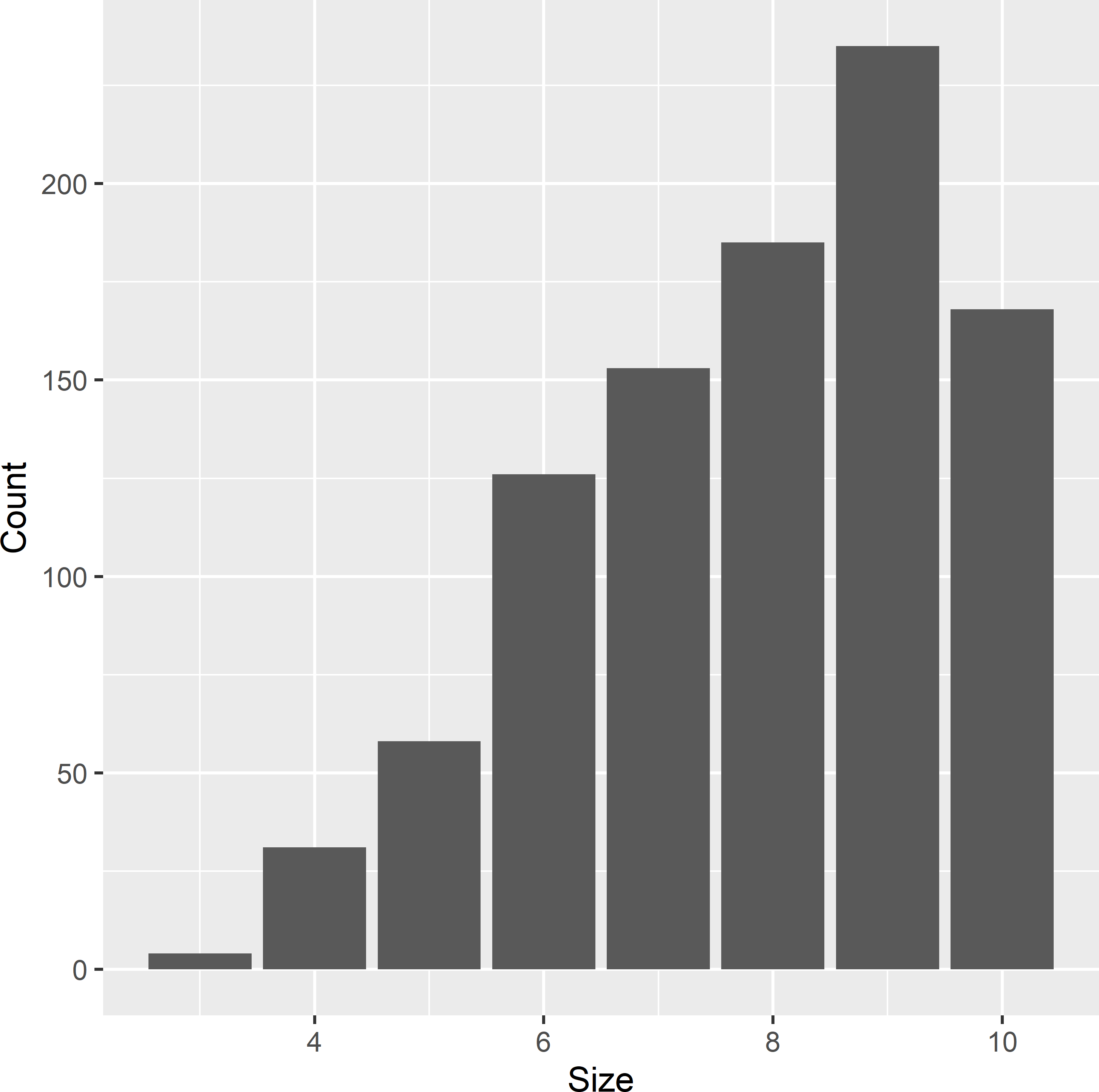

Frequency distribution of the size of clusters in Voorst. Clusters are E-W oriented transects within zones, with a spacing of 100 m between units.

Figure 6.1: Frequency distribution of the size of clusters in Voorst. Clusters are E-W oriented transects within zones, with a spacing of 100 m between units.

In total, there are 960 clusters in the population. Figure 6.1 shows the frequency distribution of the size of the clusters.

Clusters are selected with probabilities proportional to their size and with replacement (ppswr). This can be done by simple random sampling with replacement of elementary units (centres of grid cells) and identifying the clusters to which these units belong. Finally, all units of the selected clusters are included in the sample. In the code chunk below, a function is defined for selecting clusters by ppswr. Note variable cldraw, that has value 1 for all units selected in the first draw, value 2 for all units selected in the second draw, etc. This variable is needed in estimating the population mean, as explained in Section 6.1.

cl_ppswr <- function(sframe, n) {
  units <- sample(nrow(sframe), size = n, replace = TRUE)
  units_cl <- sframe$cluster[units]
  mysamples <- NULL
  for (i in seq_len(length(units_cl))) {
    mysample <- sframe[sframe$cluster %in% units_cl[i], ]
    mysample$start <- 0
    mysample$start[mysample$unit %in% units[i]] <- 1
    mysample$cldraw <- rep(i, nrow(mysample))
    mysamples <- rbind(mysamples, mysample)
  }
  mysamples
}

Function cl_ppswr is now used to select six times a cluster by ppswr.

n <- 6
set.seed(314)
mysample <- cl_ppswr(sframe = grdVoorst, n = n)

As our population actually is infinite, the centres of the selected grid cells are jittered to a random point within the selected grid cells. Note that the same noise is added to all units of a given cluster.

mysample <- mysample %>%
  group_by(cldraw) %>%
  mutate(s1 = s1 + runif(1, min = -12.5, max = 12.5),
         s2 = s2 + runif(1, min = -12.5, max = 12.5))

Figure 6.2 shows the selected sample. Note that in this case the second west-most zone has two transects (clusters), whereas one zone has none, showing that the zones are not used as strata. The total number of selected points equals 50. Similar to systematic random sampling, with cluster random sampling the total sample size is random, so that we do not have perfect control of the total sample size. This is because in this case the size, i.e., the number of points, of the clusters is not constant but varies.

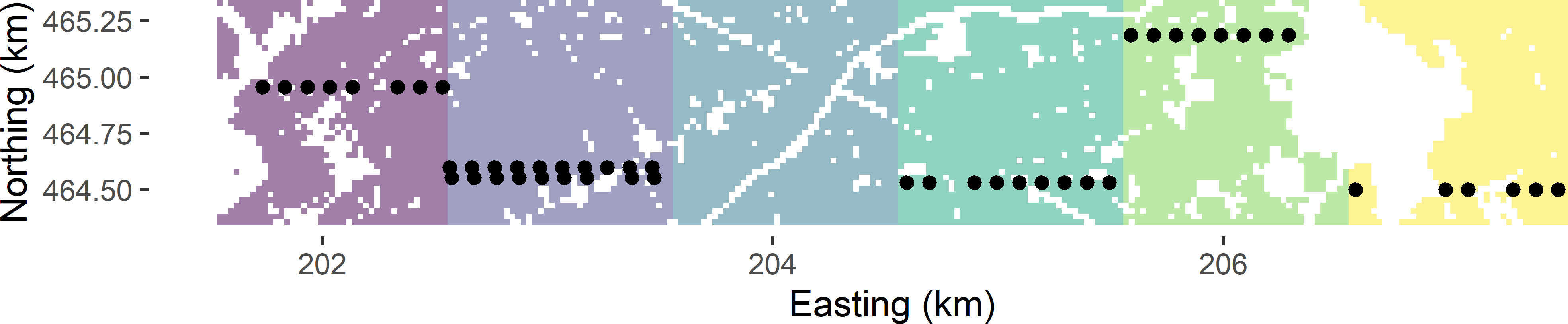
Figure 6.2: Cluster random sample from Voorst selected by ppswr.

The output data frame of function cl has a variable named start. This is an indicator with value 1 if this point of the cluster is selected first, and 0 otherwise. When in the field, it appears that the first selected point of a cluster does not belong to the target population, all other points of that cluster are also discarded. This is to keep the selection probabilities of the clusters exactly proportional to their size. Column cldraw is needed in estimation because clusters are selected with replacement. In case a cluster is selected more than once, multiple means of that cluster are used in estimation, see next section.

6.1 Estimation of population parameters

With ppswr sampling of clusters, the population total can be estimated by the pwr estimator:

\[\begin{equation} \hat{t}(z) = \frac{1}{n}\sum_{j \in \mathcal{S}} \frac{t_{j}(z)}{p_{j}} \;, \tag{6.1} \end{equation}\]

with $n$ the number of cluster draws, $p_j$ the draw-by-draw selection probability of cluster $j$, and $t_j(z)$ the total of cluster $j$:

\[\begin{equation} t_j(z) = \sum_{k=1}^{M_j} z_{kj} \;, \tag{6.2} \end{equation}\]

with $M_j$ the size (number of units) of cluster $j$ and $z_{kj}$ the study variable value of unit $k$ in cluster $j$.

The draw-by-draw selection probability of a cluster equals

\[\begin{equation} p_{j} = \frac{M_j}{M} \;, \tag{6.3} \end{equation}\]

with $M$ the total number of population units (for Voorst $M$ equals 7,528). Inserting this in Equation (6.1) yields

\[\begin{equation} \hat{t}(z) = \frac{M}{n} \sum_{j \in \mathcal{S}} \frac{t_{j}(z)}{M_{j}} = \frac{M}{n} \sum_{j \in \mathcal{S}} \bar{z}_{j} \;, \tag{6.4} \end{equation}\]

with $\bar{z}_{j}$ the mean of cluster $j$. Note that if a cluster is selected more than once, multiple means of that cluster are used in the estimator.

Dividing this estimator by the total number of population units, $M$, yields the estimator of the population mean:

\[\begin{equation} \hat{\bar{\bar{z}}}=\frac{1}{n}\sum\limits_{j \in \mathcal{S}} \bar{z}_{j} \;. \tag{6.5} \end{equation}\]

Note the two bars in $\hat{\bar{\bar{z}}}$, indicating that the observations are averaged twice.

For an infinite population of points discretised by the centres of a finite number of grid cells, $z_{kj}$ in Equation (6.2) is the study variable value at a randomly selected point within the grid cell multiplied by the area of the grid cell. The estimated population total thus obtained is equal to the estimated population mean (Equation (6.5)) multiplied by the area of the study area.

The sampling variance of the estimator of the mean with ppswr sampling of clusters is equal to (Cochran (1977), equation (9A.6))

\[\begin{equation} V(\hat{\bar{\bar{z}}})= \frac{1}{n}\sum_{j=1}^N \frac{M_j}{M} (\bar{z}_j-\bar{z})^2 \;, \tag{6.6} \end{equation}\]

with $N$ the total number of clusters (for Voorst, $N=960$), $\bar{z}_j$ the mean of cluster $j$, and $\bar{z}$ the population mean. Note that $M_j/M$ is the selection probability of cluster $j$.

This sampling variance can be estimated by (Cochran (1977), equation (9A.22))

\[\begin{equation} \widehat{V}\!\left(\hat{\bar{\bar{z}}}\right)=\frac{\widehat{S^2}(\bar{z})}{n} \;, \tag{6.7} \end{equation}\]

where $\widehat{S^2}(\bar{z})$ is the estimated variance of cluster means (the between-cluster variance):

\[\begin{equation} \widehat{S^2}(\bar{z}) = \frac{1}{n-1}\sum_{j \in \mathcal{S}}(\bar{z}_{j}-\hat{\bar{\bar{z}}})^2 \;. \tag{6.8} \end{equation}\]

In R the population mean and the sampling variance of the estimator of the population means can be estimated as follows.

est <- mysample %>%
  group_by(cldraw) %>%
  summarise(mz_cl = mean(z)) %>%
  summarise(mz = mean(mz_cl),
            se_mz = sqrt(var(mz_cl) / n()))

The estimated mean equals 87.1 g kg^-1, and the estimated standard error equals 17.4 g kg^-1. Note that the size of the clusters does not appear in these formulas. This simplicity is due to the fact that the clusters are selected with probabilities proportional to size. The effect of the cluster size on the variance is implicitly accounted for. To understand this, consider that larger clusters result in smaller variance among their means.

The same estimates are obtained with functions svydesign and svymean of package survey (Lumley 2021). Argument weights specifies the weights of the sampled clusters equal to $M/(M_j\; n)$ (Equation (6.4)).

library(survey)
M <- nrow(grdVoorst)
mysample$weights <- M / (M_cl[mysample$cluster] * n)
design_cluster <- svydesign(id = ~ cldraw, weights = ~ weights, data = mysample)
svymean(~ z, design_cluster, deff = "replace")

    mean     SE   DEff
z 87.077 17.428 4.0767

The design effect DEff as estimated from the selected cluster sample is considerably larger than 1. About 4 times more sampling points are needed with cluster random sampling compared to simple random sampling to estimate the population mean with the same precision.

A confidence interval estimate of the population mean can be computed with method confint. The number of degrees of freedom equals the number of cluster draws minus 1.

confint(svymean(~ z, design_cluster, df = degf(design_cluster), level = 0.95))

     2.5 %   97.5 %
z 52.91908 121.2347

Figure 6.3 shows the approximated sampling distribution of the pwr estimator of the mean soil organic matter (SOM) concentration with cluster random sampling and of the $\pi$ estimator with simple random sampling, obtained by repeating the random sampling with each design and estimation 10,000 times. The size of the simple random samples is equal to the expected sample size of the cluster random sampling design (rounded to nearest integer).

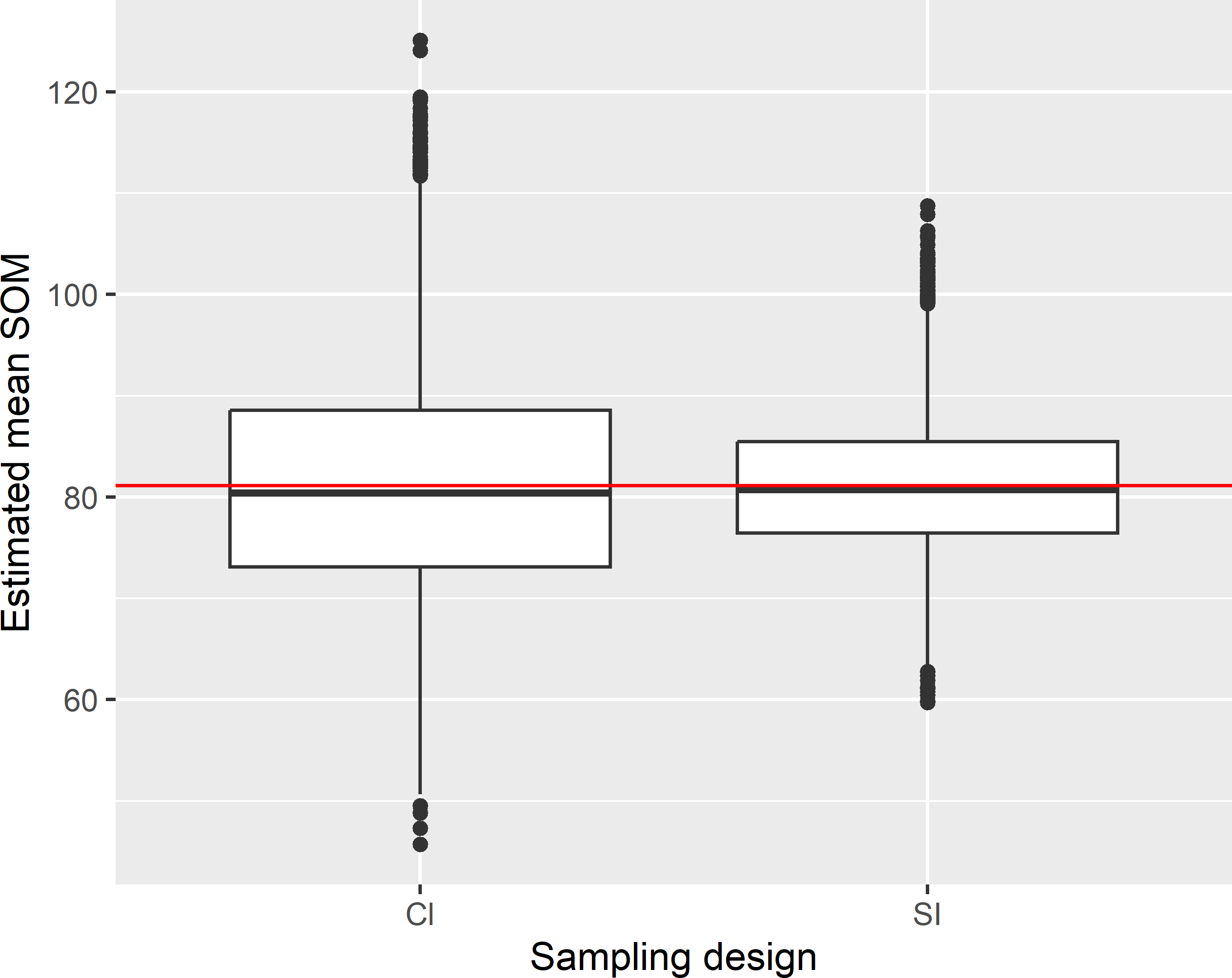
$Approximated sampling distribution of the pwr estimator of the mean SOM concentration (g kg-1) in Voorst with cluster random sampling (Cl) and of the $\pi$ estimator with simple random sampling (SI). In Cl six clusters are selected by ppswr. In SI 49 units are selected, which is equal to the expected sample size of Cl.$

Figure 6.3: Approximated sampling distribution of the pwr estimator of the mean SOM concentration (g kg^-1) in Voorst with cluster random sampling (Cl) and of the $\pi$ estimator with simple random sampling (SI). In Cl six clusters are selected by ppswr. In SI 49 units are selected, which is equal to the expected sample size of Cl.

The variance of the 10,000 estimated population means with cluster random sampling equals 126.2 (g kg^-1)². This is considerably larger than with simple random sampling: 44.8 (g kg^-1)². The large variance is caused by the strong spatial clustering of points. This may save travel time in large study areas, but in Voorst the saved travel time will be very limited, and therefore cluster random sampling in Voorst is not a good idea. The average of the estimated variances with cluster random sampling equals 125.9 (g kg^-1)². The difference with the variance of the 10,000 estimated means is small because the estimator of the variance, Equation (6.7), is unbiased. Figure 6.4 shows the approximated sampling distribution of the sample size. The expected sample size can be computed as follows:

p <- M_cl / sum(M_cl)
print(m_n <- n * sum(p * M_cl))

[1] 49.16844

So, the unequal draw-by-draw selection probabilities of the clusters are accounted for in computing the expected sample size.

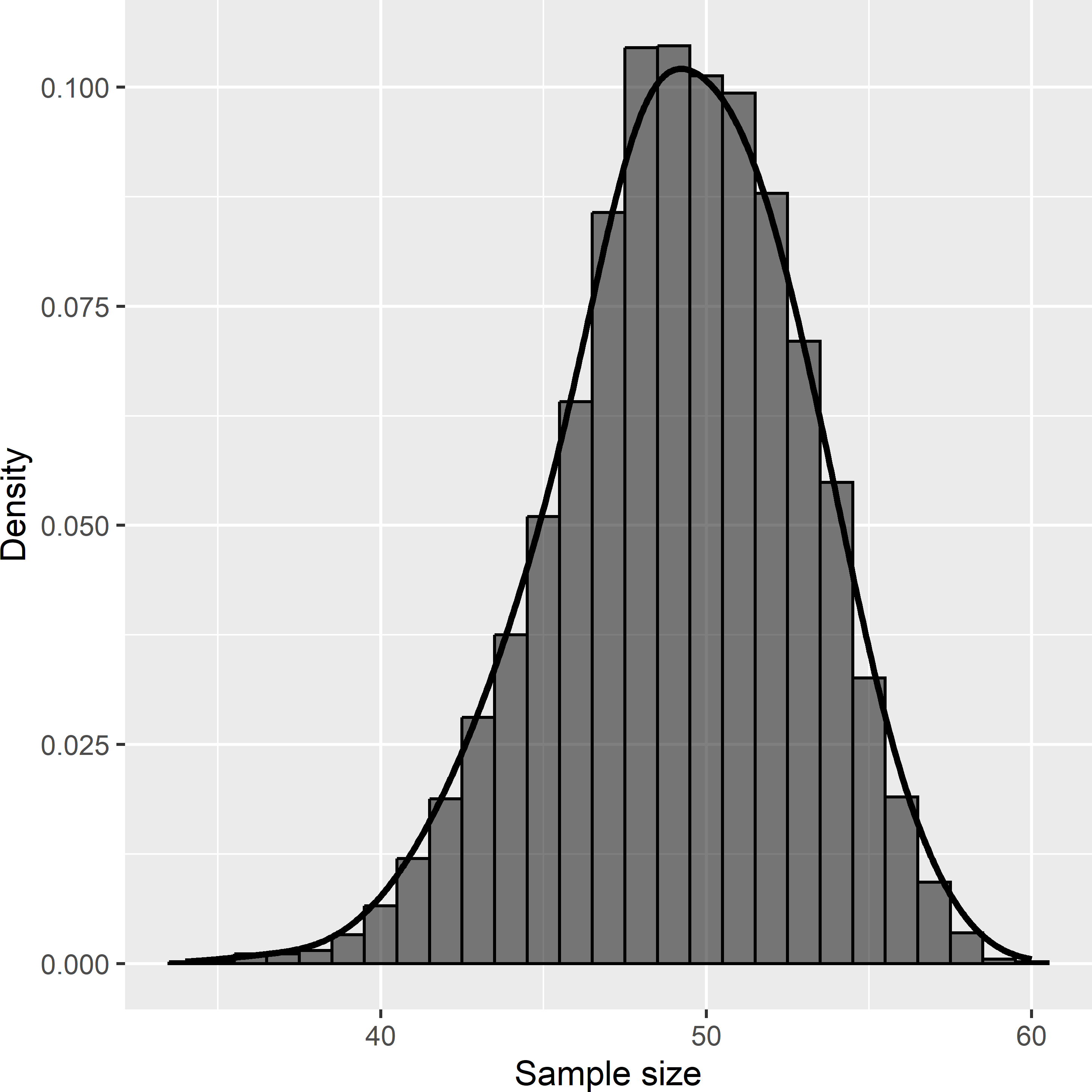
Figure 6.4: Approximated sampling distribution of the sample size with cluster random sampling from Voorst, for six clusters selected by ppswr.

Exercises

Write an R script to compute the true sampling variance of the estimator of the mean SOM concentration in Voorst for cluster random sampling and clusters selected with ppswr, $n = 6$, see Equation (6.6). Compare the sampling variance for cluster random sampling with the sampling variance for simple random sampling with a sample size equal to the expected sample size of cluster random sampling.
As an alternative we may select three times a transect, using three 2 km $\times$ 1 km zones obtained by joining two neighbouring 1 km $\times$ 1 km zones of Figure 6.2. Do you expect that the sampling variance of the estimator of the population mean is equal to, larger or smaller than that of the sampling design with six transects of half the length?

6.2 Clusters selected with probabilities proportional to size, without replacement

In the previous section the clusters were selected with replacement (ppswr). The advantage of sampling with replacement is that this keeps the statistical inference simple, more specifically the estimation of the standard error of the estimator of the population mean. However, in sampling from finite populations, cluster sampling with replacement is less efficient than cluster sampling without replacement, especially with large sampling fractions of clusters, i.e., if $1-n/N$ is small, with $N$ being the total number of clusters and $n$ the sample size, i.e., the number of cluster draws. If a cluster is selected more than once, there is less information about the population mean in this sample than in a sample with all clusters different. Selection of clusters with probabilities proportional to size without replacement (ppswor) is not straightforward.

The problem is the computation of the inclusion probabilities of the clusters. After we have selected a first cluster, we must adapt the sum of the sizes of the $N-1$ remaining clusters and recompute the selection probabilities of the remaining clusters in the second draw, etc. Section 6.4 of Lohr (1999) nicely describes how the inclusion probabilities of the $N$ clusters in a cluster random sample of size two, selected by ppswor, can be computed.

Many algorithms have been developed for ppswor sampling, see Tillé (2006) for an overview, and quite a few of them are implemented in package sampling (Tillé and Matei 2021). In the next code chunk, function UPpivotal is used to select a cluster random sample with ppswor. For an explanation of this algorithm, see Subsection 8.2.2.

library(sampling)
n <- 6
pi <- n * M_cl / M
set.seed(314)
eps <- 1e-6
sampleind <- UPpivotal(pik = pi, eps = eps)
clusters <- sort(unique(grdVoorst$cluster))
clusters_sampled <- clusters[sampleind == 1]
mysample <- grdVoorst[grdVoorst$cluster %in% clusters_sampled, ]

All inclusion probabilities pi are smaller than 1. However, this is not guaranteed when computed as in the code chunk above. In case there are units whose size is an extreme positive outlier, the inclusion probabilities of these units can become larger than 1. These units then are always selected. The inclusion probabilities of the remaining units must be recomputed, using a reduced sample size and the sizes of the remaining units. This is what is done with function inclusionprobabilities of package sampling.

The population mean can be estimated by the $\pi$ estimator by writing a few lines of R code yourself or by using function svymean of package survey as shown hereafter. Estimation of the sampling variance in pps sampling of clusters without replacement is difficult³. A simple solution is to treat the cluster sample as a ppswr sample and to estimate the variance with Equation (6.7). With small sampling fractions, this variance approximation is fine: the overestimation of the variance is negligible. For larger sampling fractions, various alternative variance approximations are developed, see Berger (2004) for details. One of the methods is Brewer’s method, which is implemented in function svydesign.

names(pi) <- clusters
mysample$pi <- pi[mysample$cluster]
design_clppswor <- svydesign(
  id = ~ cluster, data = mysample, pps = "brewer", probs = ~ pi, fpc = ~ pi)
svymean(~ z, design_clppswor)

   mean     SE
z 96.83 13.454

Another variance estimator implemented in function svydesign is the Hartley-Rao estimator. The two estimated standard errors are nearly equal.

p2sum <- sum((n * M_cl[mysample$cluster] / M)^2) / n
design_hr <- svydesign(
  id = ~ cluster,  data = mysample, pps = HR(p2sum), probs = ~ pi, fpc = ~ pi)
svymean(~ z, design_hr)

   mean     SE
z 96.83 13.436

6.3 Simple random sampling of clusters

Suppose the clusters have unequal size, but we do not know the size of the clusters, so that we cannot select the clusters with probabilities proportional to their size. In this case, we may select the clusters by simple random sampling without replacement. The inclusion probability of a cluster equals $n/N$ with $n$ the number of selected clusters and $N$ the total number of clusters in the population. This yields the following $\pi$ estimator of the population total:

\[\begin{equation} \hat{t}(z) = \frac{N}{n} \sum_{j \in \mathcal{S}} t_{j}(z)\;. \tag{6.9} \end{equation}\]

The population mean can be estimated by dividing this estimator of the population total by the total number of units in the population $M$:

\[\begin{equation} \hat{\bar{\bar{z}}}_{\pi}(z) = \frac{\hat{t}(z)}{M}\;. \tag{6.10} \end{equation}\]

Alternatively, we may estimate the population mean by dividing the estimate of the population total by the estimated population size:

\[\begin{equation} \widehat{M} = \sum_{j \in \mathcal{S}} \frac{M_{j}}{\pi_{j}} = \frac{N}{n} \sum_{j \in \mathcal{S}} M_{j} \;. \tag{6.11} \end{equation}\]

This leads to the ratio estimator of the population mean:

\[\begin{equation} \hat{\bar{\bar{z}}}_{\text{ratio}}(z) = \frac{\hat{t}(z)}{\widehat{M}} \;. \tag{6.12} \end{equation}\]

The $\pi$ estimator and the ratio estimator are equal when the clusters are selected with probabilities proportional to size. This is because the estimated population size is equal to the true population size.

print(M_HT <- sum(1 / mysample$pi))

[1] 7528

However, when clusters of different size are selected with equal probabilities, the two estimators are different. This is shown below. Six clusters are selected by simple random sampling without replacement.

set.seed(314)
clusters <- sort(unique(grdVoorst$cluster))
units_cl <- sample(length(clusters), size = n, replace = FALSE)
clusters_sampled <- clusters[units_cl]
mysample <- grdVoorst[grdVoorst$cluster %in% clusters_sampled, ]

The $\pi$ estimate and the ratio estimate of the population mean are computed for the selected sample.

N <- length(clusters)
mysample$pi <- n / N
tz_HT <- sum(mysample$z / mysample$pi)
mz_HT <- tz_HT / M
M_HT <- sum(1 / mysample$pi)
mz_ratio <- tz_HT / M_HT

The $\pi$ estimate equals 68.750 g kg^-1, and the ratio estimate equals 70.319 g kg^-1. The $\pi$ estimate of the population mean can also be computed by first computing totals of clusters, see Equations (6.9) and (6.10).

tz_cluster <- tapply(mysample$z, INDEX = mysample$cluster, FUN = sum)
pi_cluster <- n / N
tz_HT <- sum(tz_cluster / pi_cluster)
print(mz_HT <- tz_HT / M)

[1] 68.74994

The variance of the $\pi$ estimator of the population mean can be estimated by first estimating the variance of the estimator of the total:

\[\begin{equation} \widehat{V}(\hat{t}(z)) = N^2\left(1-\frac{n}{N}\right)\frac{\widehat{S^2}(t(z))}{n} \tag{6.13} \;, \end{equation}\]

and dividing this variance by the squared number of population units:

\[\begin{equation} \widehat{V}(\hat{\bar{\bar{z}}}) = \frac{1}{M^2} \widehat{V}(\hat{t}(z)) \;. \tag{6.14} \end{equation}\]

fpc <- 1 - n / N
v_tz <- N^2 * fpc * var(tz_cluster) / n
se_mz_HT <- sqrt(v_tz / M^2)

The estimated standard error equals 11.5 g kg^-1.

To compute the variance of the ratio estimator of the population mean, we first compute residuals of cluster totals:

\[\begin{equation} e_j = t_j(z)-\hat{b}M_j \;, \tag{6.15} \end{equation}\]

with $\hat{b}$ the ratio of the estimated population mean of the cluster totals to the estimated population mean of the cluster sizes:

\[\begin{equation} \hat{b}=\frac{\frac{1}{n}\sum_{j \in \mathcal{S}} t_{j}}{\frac{1}{n}\sum_{j \in \mathcal{S}} M_{j}} \;. \tag{6.16} \end{equation}\]

The variance of the ratio estimator of the population mean can be estimated by

\[\begin{equation} \hat{V}(\hat{\bar{\bar{z}}}_{\text{ratio}})=\left(1-\frac{n}{N}\right)\frac{1}{(\frac{1}{n}\sum_{j \in \mathcal{S}} M_{j})^2}\frac{\widehat{S^2}_e}{n} \;, \tag{6.17} \end{equation}\]

with $\widehat{S^2}_e$ the estimated variance of the residuals.

m_M_cl <- mean(M_cl[unique(mysample$cluster)])
b <- mean(tz_cluster) / m_M_cl
e_cl <- tz_cluster - b * M_cl[sort(unique(mysample$cluster))]
S2e <- var(e_cl)
print(se_mz_ratio <- sqrt(fpc * 1 / m_M_cl^2 * S2e / n))

[1] 12.39371

The ratio estimate can also be computed with function svymean of package survey, which also provides an estimate of the standard error of the estimated mean.

design_SIC <- svydesign(
  id = ~ cluster, probs = ~ pi, fpc = ~ pi, data = mysample)
svymean(~ z, design_SIC)

    mean     SE
z 70.319 12.394

6.4 Stratified cluster random sampling

The basic sampling designs stratified random sampling (Chapter 4) and cluster random sampling can be combined into stratified cluster random sampling. So, instead of selecting simple random samples from the strata, within each stratum clusters are randomly selected. Figure 6.5 shows a stratified cluster random sample from Voorst. The strata consist of three 2 km $\times$ 1 km zones, obtained by joining two neighbouring 1 km $\times$ 1 km zones (Figure 6.2). The clusters are the same as before, i.e., E-W oriented transects within 1 km $\times$ 1 km zones, with an inter-unit spacing of 100 m. Within each stratum, two times a cluster is selected by ppswr. The stratification avoids the clustering of the selected transects in one part of the study area. Compared to (unstratified) cluster random sampling, the geographical spreading of the clusters is improved, which may lead to an increase of the precision of the estimated population mean. In Figure 6.5 and in the most western stratum, the two selected transects are in the same 1 km $\times$ 1 km zone. The alternative would be to use the six zones as strata, leading to an improved spreading of the clusters, but there is also a downside with this design, see Exercise 3. Note that the selection probabilities are now equal to

\[\begin{equation} p_{jh}= M_j/M_h \;, \tag{6.18} \end{equation}\] with $M_h$ the total number of population units of stratum $h$.

grdVoorst$zone_stratum <- as.factor(grdVoorst$zone)
levels(grdVoorst$zone_stratum) <- rep(c("a", "b", "c"), each = 2)
n_h <- c(2, 2, 2)
set.seed(324)
stratumlabels <- unique(grdVoorst$zone_stratum)
mysample <- NULL
for (i in 1:3) {
  grd_h <- grdVoorst[grdVoorst$zone_stratum == stratumlabels[i], ]
  mysample_h <- cl_ppswr(sframe = grd_h, n = n_h[i])
  mysample <- rbind(mysample, mysample_h)
}

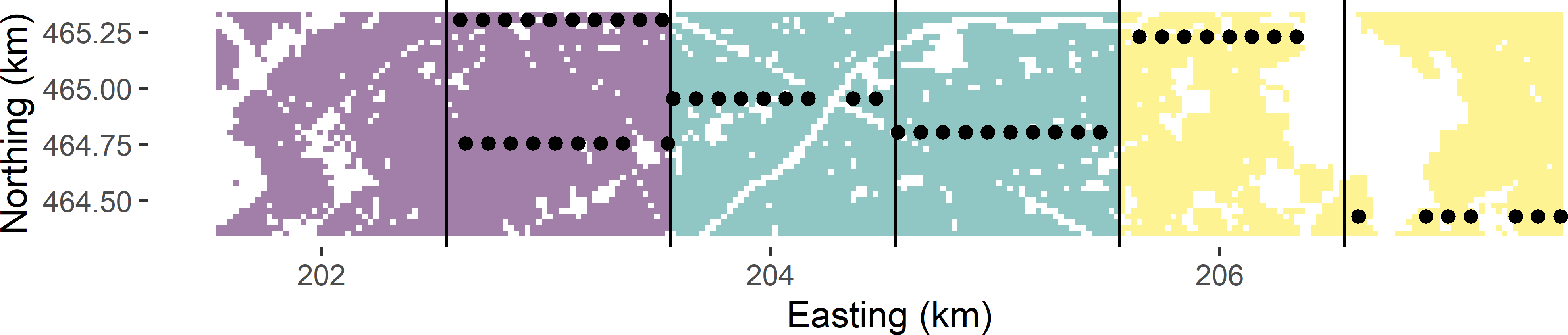
Figure 6.5: Stratified cluster random sample from Voorst, with three strata. From each stratum two times a cluster is selected by ppswr.

The population mean is estimated by first estimating the stratum means using Equation (6.5) at the level of the strata, followed by computing the weighted average of the estimated stratum means using Equation (4.3). The variance of the estimator of the population mean is estimated in the same way, by first estimating the variance of the estimator of the stratum means using Equations (6.7) and (6.8) at the level of the strata, followed by computing the weighted average of the estimated variances of the estimated stratum means (Equation (4.4)).

strata_size <- grdVoorst %>%
  group_by(zone_stratum) %>%
  summarise(M_h = n()) %>%
  mutate(w_h = M_h / sum(M_h))
est <- mysample %>%
  group_by(zone_stratum, cldraw) %>%
  summarise(mz_cl = mean(z), .groups = "drop_last") %>%
  summarise(mz_h = mean(mz_cl),
            v_mz_h = var(mz_cl) / n()) %>%
  left_join(strata_size, by = "zone_stratum") %>%
  summarise(mz = sum(w_h * mz_h),
            se_mz = sqrt(sum(w_h^2 * v_mz_h)))

The estimated mean equals 82.8 g kg^-1, and the estimated standard error equals 4.7 g kg^-1. The same estimates are obtained with function svymean. Weights for the clusters are computed as before, but now at the level of the strata. Note argument nest = TRUE, which means that the clusters are nested within the strata.

mysample$weights <- strata_size$M_h[mysample$zone_stratum] /
  (M_cl[mysample$cluster] * n_h[mysample$zone_stratum])
design_strcluster <- svydesign(id = ~ cldraw, strata = ~ zone_stratum,
  weights = ~ weights, data = mysample, nest = TRUE)
svymean(~ z, design_strcluster)

    mean     SE
z 82.796 4.6737

Exercises

Why is it attractive in stratified random cluster sampling to select at least two clusters per stratum?

References

Berger, Y. G. 2004. “A Simple Variance Estimator for Unequal Probability Sampling Without Replacement.” Canadian Journal of Applied Statistics 31 (3): 305–15. https://doi.org/10.1080/0266476042000184046.

Cochran, W. G. 1977. Sampling Techniques. New York: Wiley.

de Gruijter, J. J., D. J. Brus, M. F. P. Bierkens, and M. Knotters. 2006. Sampling for Natural Resource Monitoring. Berlin: Springer.

Lohr, S. L. 1999. Sampling: Design and Analysis. Pacific Grove: Duxbury Press.

———. 2021. survey: Analysis of Complex Survey Samples.

Tillé, Y. 2006. Sampling Algorithms. New York: Springer.

Tillé, Y., and A. Matei. 2021. sampling: Survey Sampling. https://CRAN.R-project.org/package=sampling.

Wickham, Hadley. 2019. Stringr: Simple, Consistent Wrappers for Common String Operations. https://CRAN.R-project.org/package=stringr.

The problem is the computation of the joint inclusion probabilities of pairs of points.↩︎