Chapter 9 Balanced and well-spread sampling
In this chapter two related but fundamentally different sampling designs are described and illustrated. The similarity and difference are shortly outlined below, but hopefully will become clearer in following sections.
Roughly speaking, for a balanced sample the sample means of covariates are equal to the population means of these covariates. When the covariates are linearly related to the study variable, this may yield a more precise estimate of the population mean or total of the study variable.
A well-spread sample is a sample with a large range of values for the covariates, from small to large values, but also including intermediate values. In more technical terms: the sampling units are well-spread along the axes spanned by the covariates. If the spatial coordinates are used as covariates (spreading variables), this results in samples that are well-spread in geographical space. Such samples are commonly referred to as spatially balanced samples, which is somewhat confusing, as the geographical spreading is not implemented through balancing on the geographical coordinates. On the other hand, the averages of the spatial coordinates of a sample well-spread in geographical space will be close to the population means of the coordinates. Therefore, the sample will be approximately balanced on the spatial coordinates (Grafström and Schelin 2014). The reverse is not true: with balanced sampling, the spreading of the sampling units in the space spanned by the balancing variables can be poor. A sample with all values of a covariate used in balancing near the population mean of that variable has a poor spreading along the covariate axis, but can still be perfectly balanced.
9.1 Balanced sampling
Balanced sampling is a sampling method that exploits one or more quantitative covariates that are related to the study variable. The idea behind balanced sampling is that, if we know the mean of the covariates, then the sampling efficiency can be increased by selecting a sample whose averages of the covariates must be equal to the population means of the covariates.
Let me illustrate balanced sampling with a small simulation study. The simulated population shown in Figure 9.1 shows a linear trend from West to East and besides a trend from South to North. Due to the West-East trend, the simulated study variable \(z\) is correlated with the covariate Easting and, due to the South-North trend, also with the covariate Northing. To estimate the population mean of the simulated study variable, intuitively it is attractive to select a sample with an average of the Easting coordinate that is equal to the population mean of Easting (which is 10). Figure 9.1 (subfigure on the left) shows such a sample of size four; we say that the sample is `balanced’ on the covariate Easting. The sample in the subfigure on the right is balanced on Easting as well as on Northing.
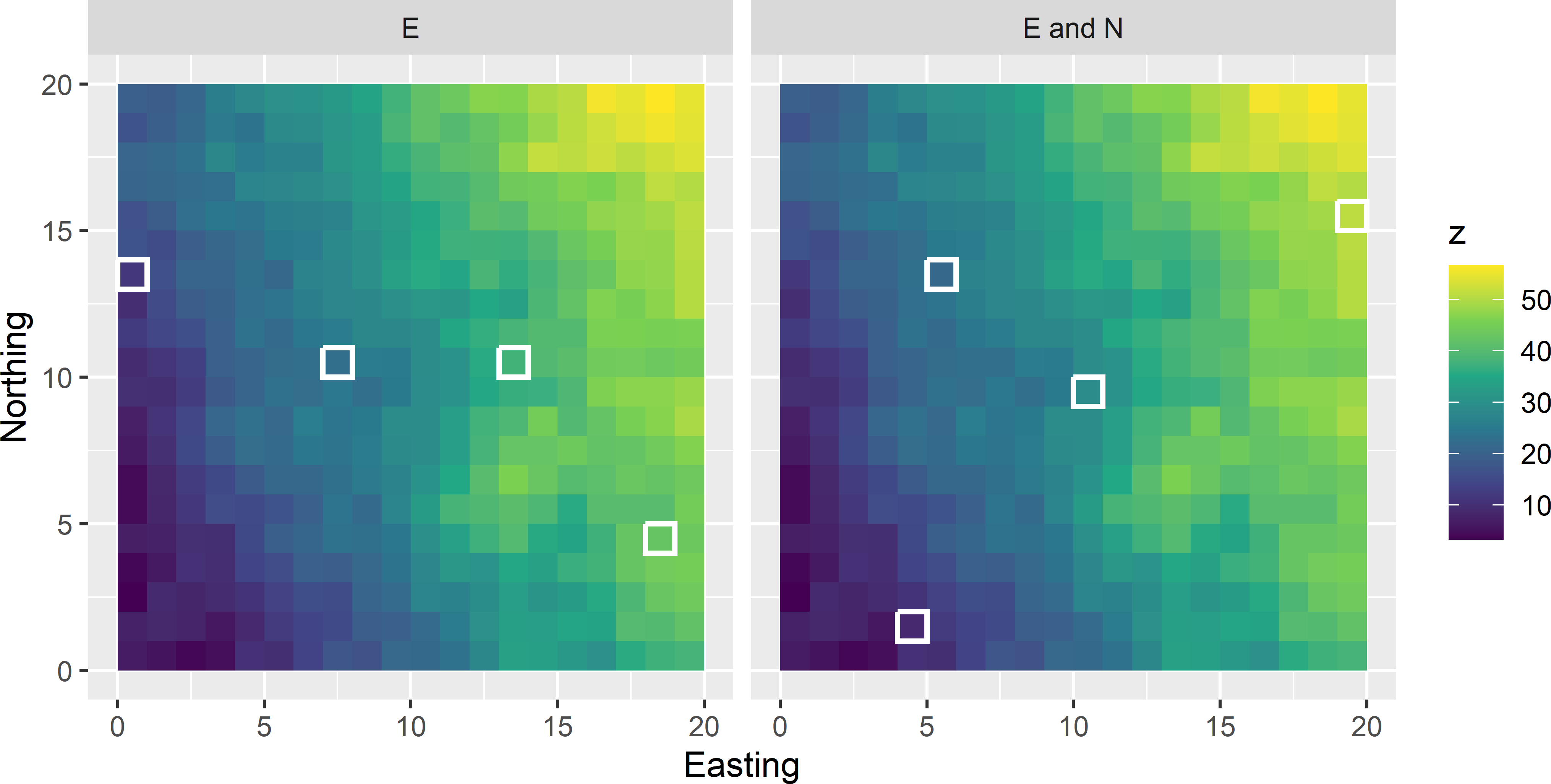
Figure 9.1: Sample balanced on Easting (E) and on Easting and Northing (E and N).
9.1.1 Balanced sample vs. balanced sampling design
We must distinguish a balanced sample from a balanced sampling design. A sampling design is balanced on a covariate \(x\) when all possible samples that can be generated by the design are balanced on \(x\).
Figure 9.2 shows for 1,000 simple random samples the squared error of the estimated population mean of the study variable \(z\) against the difference between the sample mean of balancing variable Easting and the population mean of Easting. Clearly, the larger the absolute value of the difference, the larger on average the squared error. So, to obtain a precise and accurate estimate of the population mean of \(z\), we better select samples with a difference close to 0.
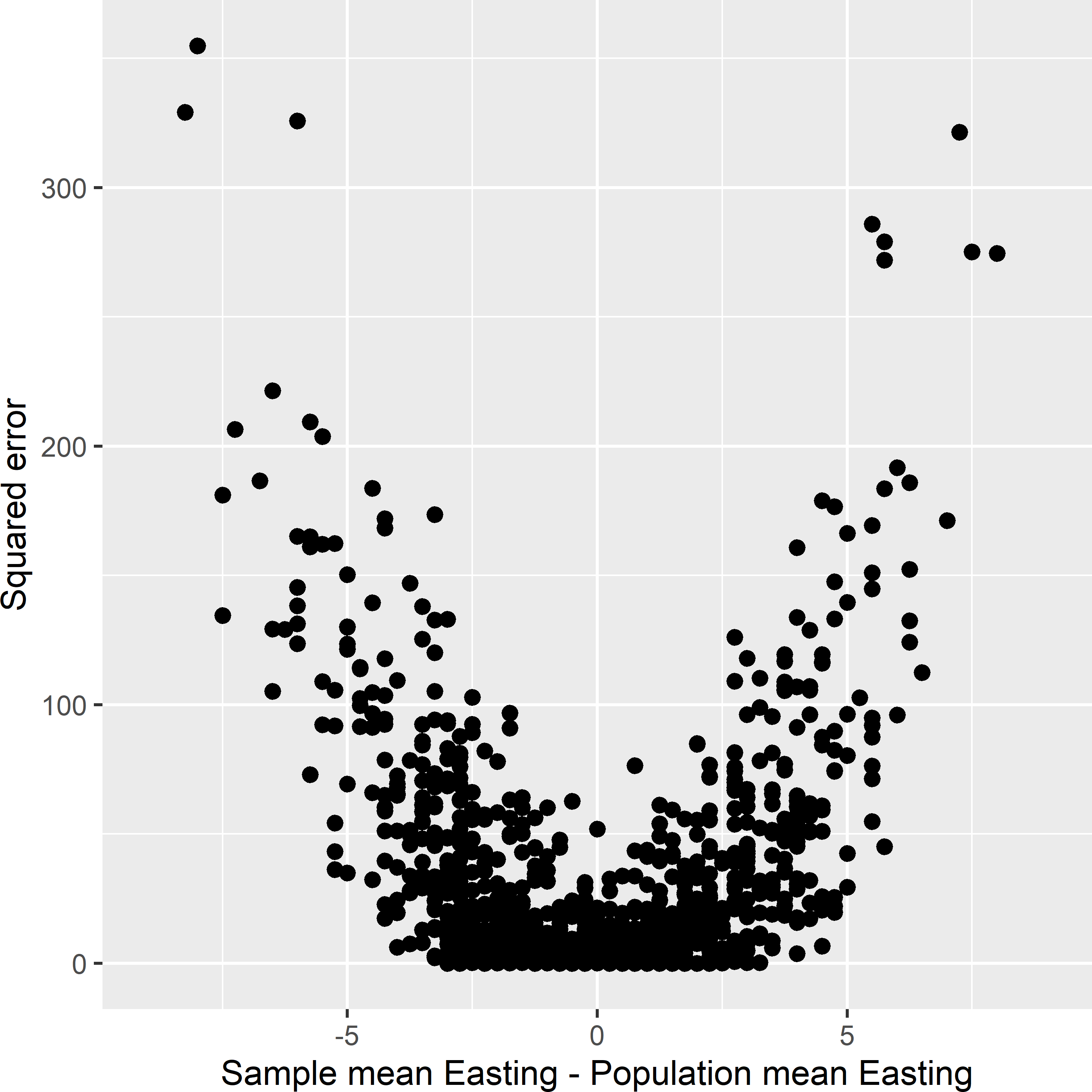
Figure 9.2: Squared error in the estimated population mean of \(z\) against the difference between the sample mean and the population mean of Easting, for 1,000 simple random samples of size four selected from the population shown in Figure 9.1.
Using only Easting as a balancing variable reduces the sampling variance of the estimator of the mean substantially. Using Easting and Northing as balancing variables further reduces the sampling variance. See Table 9.1.
| Sampling design | Balancing variables | Sampling variance |
|---|---|---|
| SI |
|
39.70 |
| Balanced | Easting | 14.40 |
| Balanced | Easting and Northing | 9.77 |
9.1.2 Unequal inclusion probabilities
Until now we have assumed that the inclusion probabilities of the population units are equal, but this is not a requirement for balanced sampling designs. A more general definition of a balanced sampling design is as follows. A sampling design is balanced on variable \(x\) when for all samples generated by the design the \(\pi\) estimate of the population total of \(x\) equals the population total of \(x\):
\[\begin{equation} \sum_{k \in \mathcal{S}} \frac{x_k}{\pi_k}= \sum_{k=1}^{N} x_k \;. \tag{9.1} \end{equation}\]
Similar to the regression estimator explained in the next chapter (Subsection 10.1.1), balanced sampling exploits the linear relation between the study variable and one or more covariates. When using the regression estimator, this is done at the estimation stage. Balanced sampling does so at the sampling stage. For a single covariate the regression estimator of the population total equals (see Equation (10.10))
\[\begin{equation} \hat{t}_{\mathrm{regr}}(z) = \hat{t}_{\pi}(z) + \hat{b}\left(t(x) - \hat{t}_{\pi}(x)\right) \;, \tag{9.2} \end{equation}\]
with \(\hat{t}_{\pi}(z)\) and \(\hat{t}_{\pi}(x)\) the \(\pi\) estimators of the population total of the study variable \(z\) and the covariate \(x\), respectively, \(t(x)\) the population total of the covariate, and \(\hat{b}\) the estimated slope parameter (see hereafter). With a perfectly balanced sample the second term in the regression estimator, which adjusts the \(\pi\) estimator, equals zero.
Balanced samples can be selected with the cube algorithm of Deville and Tillé (2004). The population total and mean can be estimated by the \(\pi\) estimator. The approximated variance of the \(\pi\) estimator of the population mean can be estimated by (Deville and Tillé (2005), Grafström and Tillé (2013))
\[\begin{equation} \widehat{V}(\hat{\bar{z}}) = \frac{1}{N^2}\frac{n}{n-p} \sum_{k \in \mathcal{S}} c_k \left(\frac{e_k}{\pi_k}\right)^2 \;, \tag{9.3} \end{equation}\]
with \(p\) the number of balancing variables, \(c_k\) a weight for unit \(k\) (see hereafter), and \(e_k\) the residual of unit \(k\) given by
\[\begin{equation} e_k = z_k - \mathbf{x}_k^{\text{T}}\hat{\mathbf{b}} \;, \tag{9.4} \end{equation}\]
with \(\mathbf{x}_k\) a vector of length \(p\) with the balancing variables for unit \(k\), and \(\hat{\mathbf{b}}\) the estimated population regression coefficients, given by
\[\begin{equation} \hat{\mathbf{b}} = \left(\sum_{k \in \mathcal{S}} c_k \frac{\mathbf{x}_k}{\pi_k} \frac{\mathbf{x}_k}{\pi_k}^{\text{T}} \right)^{-1} \sum_{k \in \mathcal{S}} c_k \frac{\mathbf{x}_k}{\pi_k} \frac{z_k}{\pi_k} \;. \tag{9.5} \end{equation}\]
Working this out for balanced sampling without replacement with equal inclusion probabilities, \(\pi_k = n/N,\; k = 1, \dots , N\), yields
\[\begin{equation} \widehat{V}(\hat{\bar{z}}) = \frac{1}{n(n-p)} \sum_{k \in \mathcal{S}} c_k e_k^2 \;. \tag{9.6} \end{equation}\]
Deville and Tillé (2005) give several formulas for computing the weights \(c_k\), one of which is \(c_k = (1-\pi_k)\).
Balanced sampling is now illustrated with aboveground biomass (AGB) data of Eastern Amazonia, see Figure 1.8. Log-transformed short-wave infrared radiation (lnSWIR2) is used as a balancing variable. The samplecube function of the sampling package (Tillé and Matei 2021) implements the cube algorithm. Argument X of this function specifies the matrix of ancillary variables on which the sample must be balanced. The first column of this matrix is filled with ones, so that the sample size is fixed. To speed up the computations, a 5 km \(\times\) 5 km subgrid of grdAmazonia is used.
Equal inclusion probabilities are used, i.e., for all population units the inclusion probability equals \(n/N\).
grdAmazonia <- grdAmazonia %>%
  mutate(lnSWIR2 = log(SWIR2))
library(sampling)
N <- nrow(grdAmazonia)
n <- 100
X <- cbind(rep(1, times = N), grdAmazonia$lnSWIR2)
pi <- rep(n / N, times = N)
sample_ind <- samplecube(X = X, pik = pi, comment = FALSE, method = 1)
eps <- 1e-6
units <- which(sample_ind > (1 - eps))
mysample <- grdAmazonia[units, ]
The population mean can be estimated by the sample mean.
To estimate the variance, a function is defined for estimating the population regression coefficients.
estimate_b <- function(z, X, c) {
  cXX <- matrix(nrow = ncol(X), ncol = ncol(X), data = 0)
  cXz <- matrix(nrow = 1, ncol = ncol(X), data = 0)
  for (i in seq_len(length(z))) {
    x <- X[i, ]
    cXX_i <- c[i] * (x %*% t(x))
    cXX <- cXX + cXX_i
    cXz_i <- c[i] * t(x) * z[i]
    cXz <- cXz + cXz_i
  }
  b <- solve(cXX, t(cXz))
  return(b)
}
The next code chunk shows how the estimated variance of the \(\pi\) estimator of the population mean can be computed.
pi <- rep(n / N, n)
c <- (1 - pi)
b <- estimate_b(z = mysample$AGB / pi, X = X[units, ] / pi, c = c)
zpred <- X %*% b
e <- mysample$AGB - zpred[units]
v_tz <- n / (n - ncol(X)) * sum(c * (e / pi)^2)
v_mz <- v_tz / N^2
Figure 9.3 shows the selected balanced sample. Note the spatial clustering of some units. The estimated population mean (as estimated by the sample mean) of AGB equals 224.5 109 kg ha-1. The population mean of AGB equals 225.3 109 kg ha-1. The standard error of the estimated mean equals 6.1 109 kg ha-1.
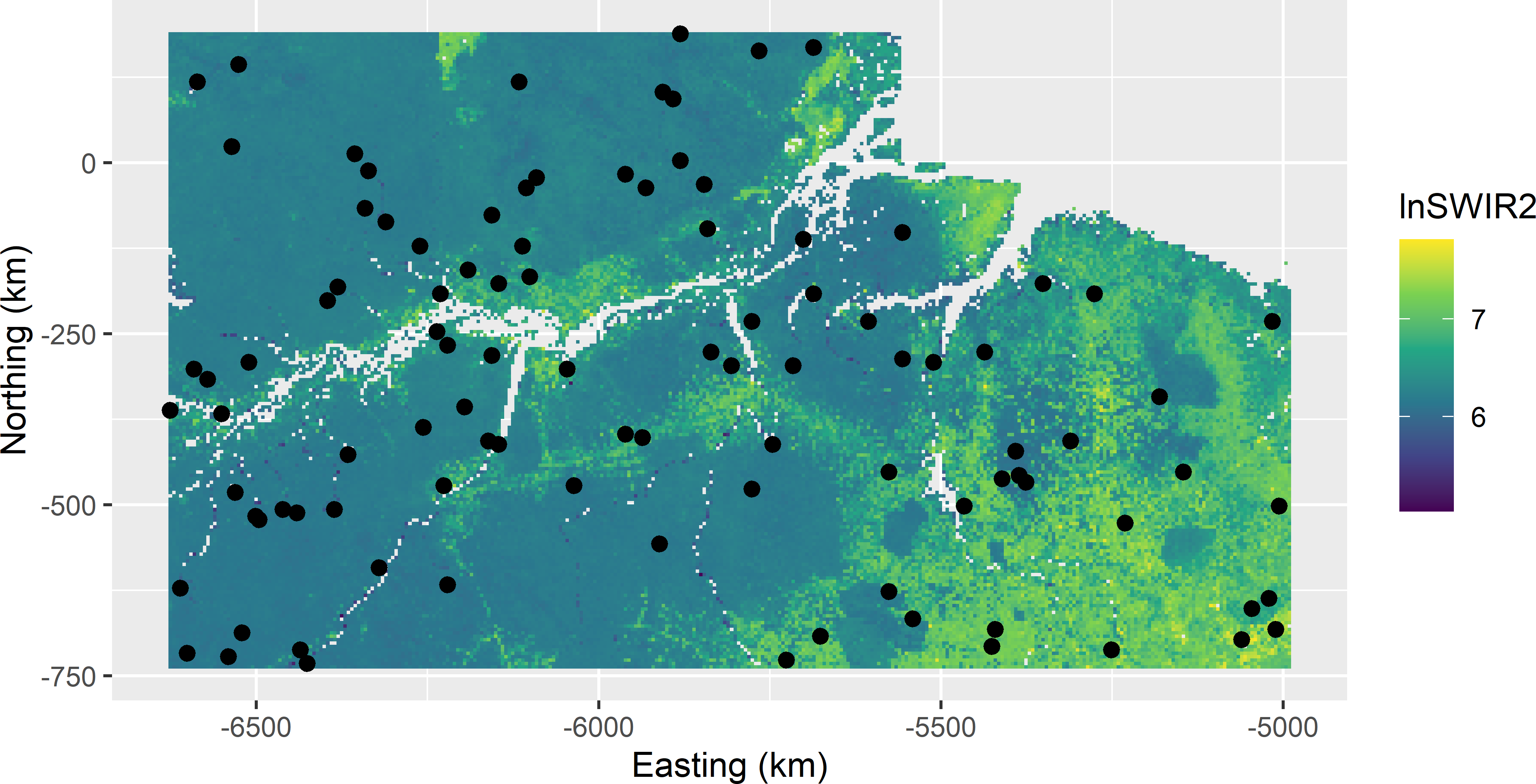
Figure 9.3: Sample balanced on lnSWIR2 from Eastern Amazonia.
Figure 9.4 shows the approximated sampling distribution of the \(\pi\) estimator of the mean AGB with balanced sampling and simple random sampling, obtained by repeating the random sampling with both designs and estimation 1,000 times.
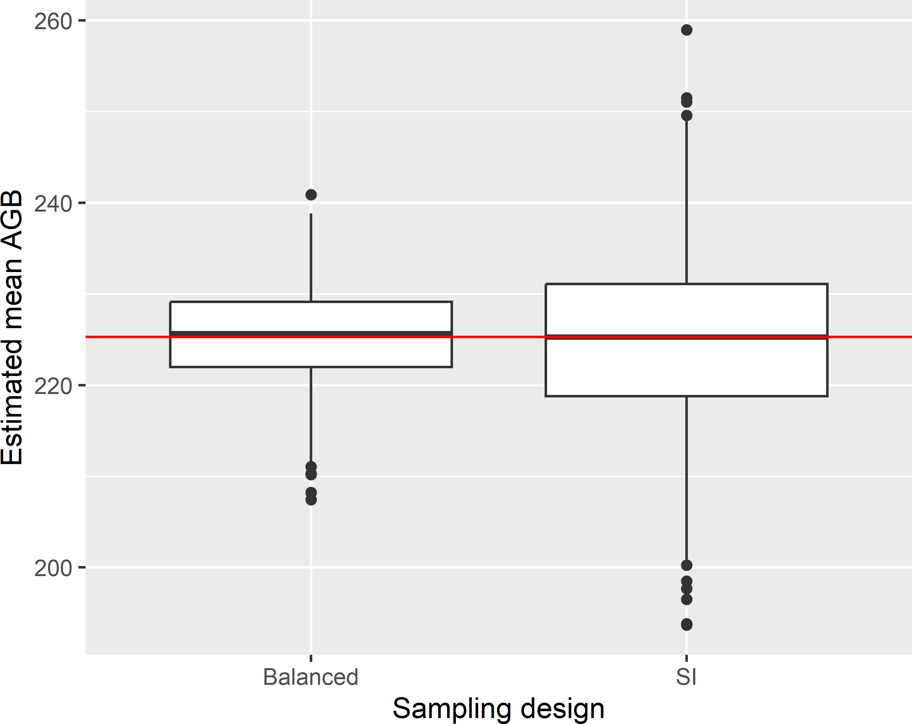
Figure 9.4: Approximated sampling distribution of the \(\pi\) estimator of the mean AGB (109 kg ha-1) in Eastern Amazonia, with balanced sampling, balanced on lnSWIR2 and using equal inclusion probabilities, and simple random sampling without replacement (SI) of 100 units.
The variance of the 1,000 estimates of the population mean of the study variable AGB equals 28.8 (109 kg ha-1)2. The gain in precision compared to simple random sampling equals 2.984 (design effect is 0.335), so with simple random sampling about three times more sampling units are needed to estimate the population mean with the same precision. The mean of the 1,000 estimated variances equals 26.4 (109 kg ha-1)2, indicating that the approximated variance estimator somewhat underestimates the true variance in this case. The population mean of the balancing variable lnSWIR2 equals 6.414. The sample mean of lnSWIR2 varies a bit among the samples. Figure 9.5 shows the approximated sampling distribution of the sample mean of lnSWIR2. In other words, many samples are not perfectly balanced on lnSWIR2. This is not exceptional; in most cases perfect balance is impossible.
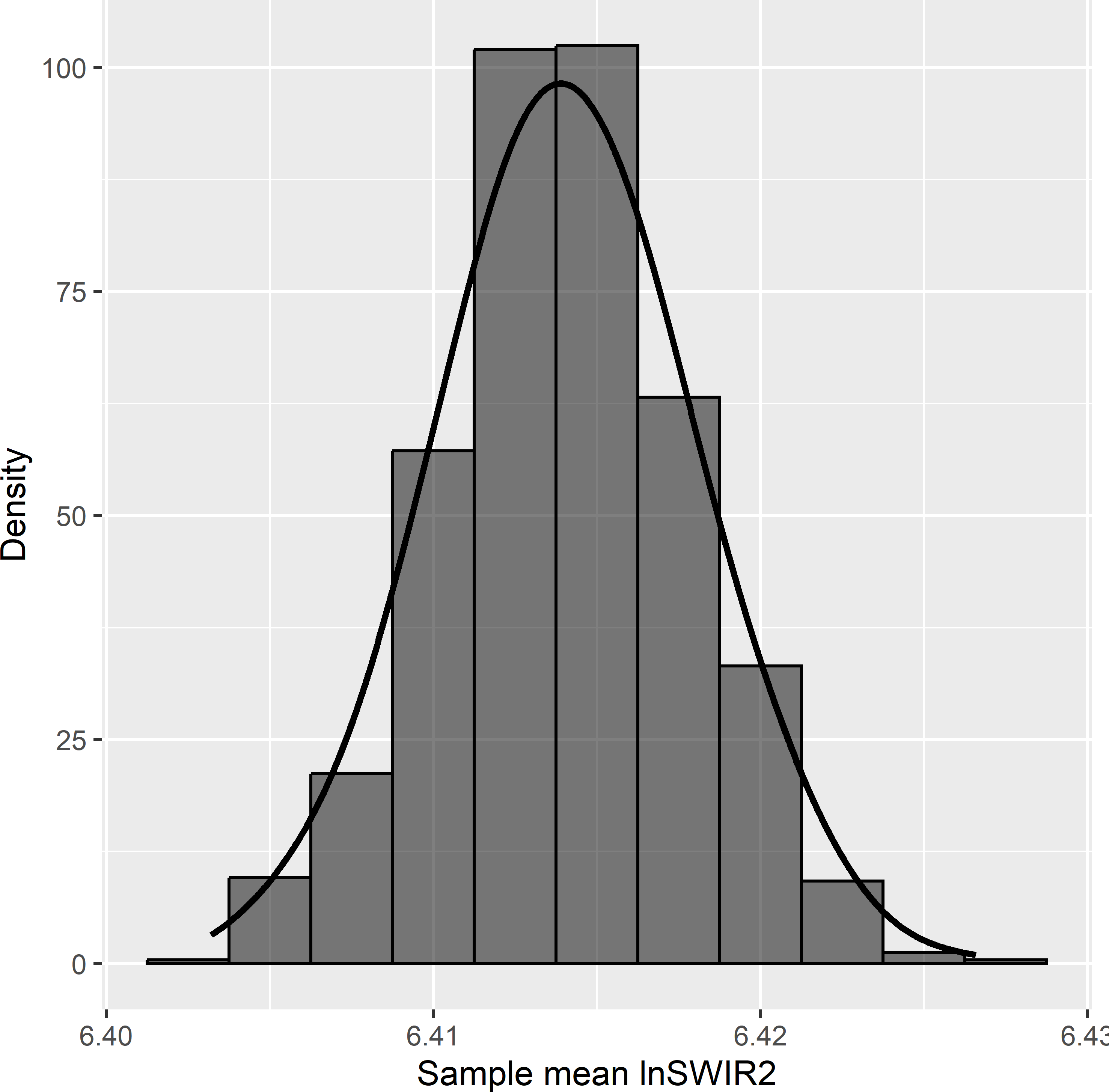
Figure 9.5: Approximated sampling distribution of the sample mean of balancing variable lnSWIR2 in Eastern Amazonia with balanced sampling of size 100 and equal inclusion probabilities.
Exercises
- Select a sample of size 100 balanced on lnSWIR2 and Terra_PP from Eastern Amazonia, using equal inclusion probabilities for all units.
- First, select a subgrid of 5 km \(\times\) 5 km using function
spsample, see Chapter 5. - Estimate the population mean.
- Estimate the standard error of the \(\pi\) estimator. First, estimate the regression coefficients, using function
estimate_bdefined above, then compute the residuals, and finally compute the variance.
- First, select a subgrid of 5 km \(\times\) 5 km using function
- Spatial clustering of sampling units is not avoided in balanced sampling. What effect do you expect of this spatial clustering on the precision of the estimated mean? Can you think of a situation where this effect does not occur?
9.1.3 Stratified random sampling
Much in the same way as we controlled in the previous subsection the sample size \(n\) by balancing the sample on the known total number of population units \(N\), we can balance a sample on the known total number of units in subpopulations. A sample balanced on the sizes of subpopulations is a stratified random sample. Figure 9.6 shows four subpopulations or strata. These four strata can be used in balanced sampling by constructing the following design matrix \(\mathbf{X}\) with as many columns as there are strata and as many rows as there are population units:
\[\begin{equation} \mathbf{X}= \begin{bmatrix} 1 &0 &0 &0 \\ 1 &0 &0 &0 \\ 1 &0 &0 &0 \\ 1 &0 &0 &0 \\ 0 &1 &0 &0 \\ 0 &1 &0 &0 \\ 0 &0 &1 &0 \\ \vdots &\vdots &\vdots &\vdots\\ 0 & 0 & 0 & 1 \\ \end{bmatrix} \;. \tag{9.7} \end{equation}\]
The first four rows refer to the four leftmost bottom row population units in Figure 9.6. These units belong to class A, which explains that the first column for these units contain ones. The other three columns for these rows contain all zeroes. The fifth and sixth unit belong to stratum B, so that the second column for these rows contain ones, and so on. The final row is the upperright sampling unit in stratum D, so the first three columns contain zeroes, and the fourth column is filled with a one. The sum of the indicators in the columns is the total number of population units in the strata.
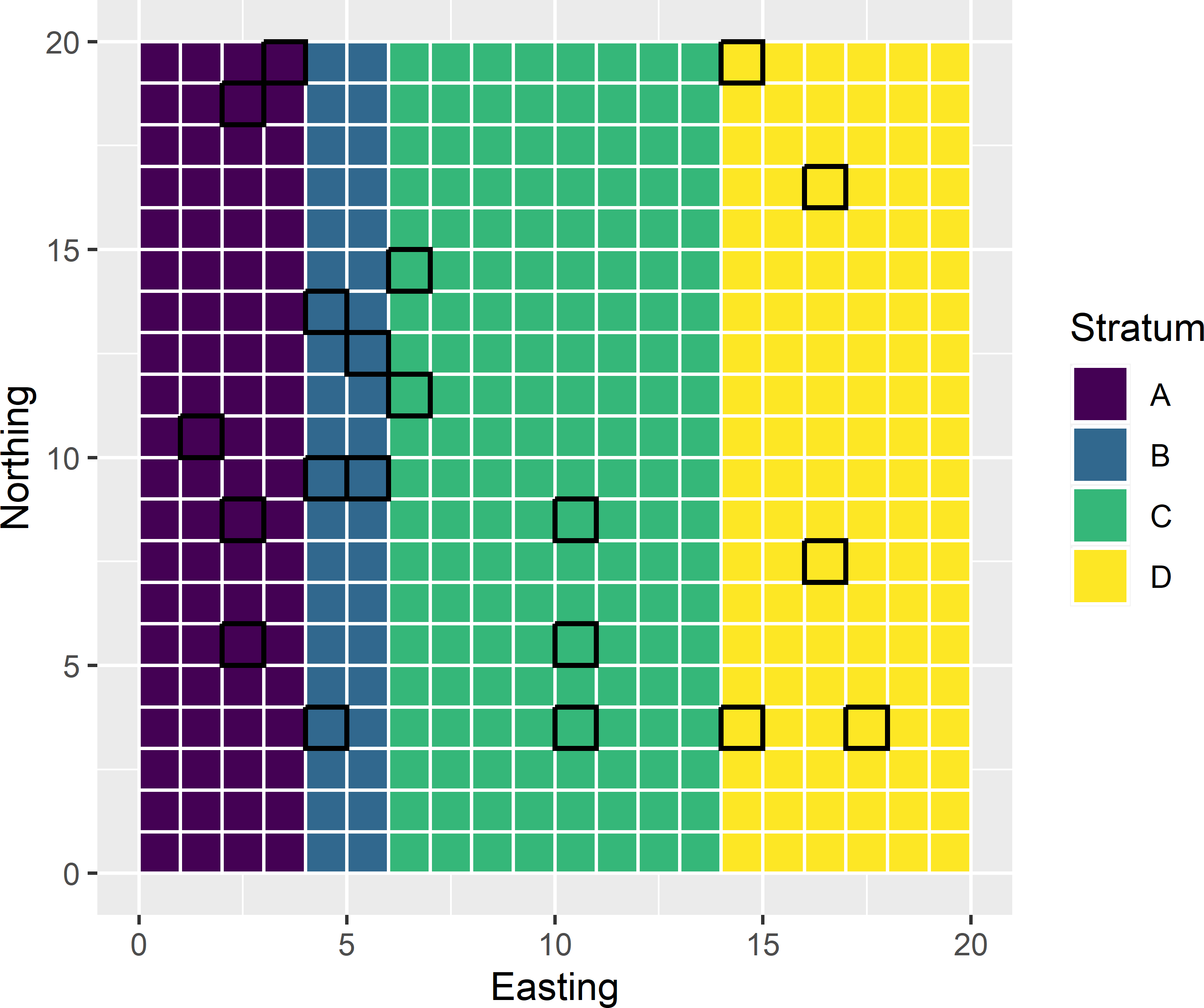
Figure 9.6: Sample balanced on a categorical variable with four classes.
In the next code chunk, the inclusion probabilities are computed by \(\pi_{hk}=n_h/N_h,\; k=1, \dots , N_h\), with \(n_h=5\) for all four strata. The stratum sample sizes are equal, but the number of population units of a stratum differ among the strata, so the inclusion probabilities also differ among the strata. The ten leftmost units on the bottom row of Figure 9.6 are shown below.
s1 <- s2 <- 1:20 - 0.5
mypop <- expand.grid(s1, s2)
names(mypop) <- c("s1", "s2")
mypop$stratum <- as.factor(findInterval(mypop$s1, c(4, 6, 14)))
levels(mypop$stratum) <- LETTERS[1:4]
mypop <- mypop %>%
    group_by(stratum) %>%
    summarise(N_h = n(), .groups = "drop") %>%
    mutate(pi_h = rep(5, 4) / N_h) %>%
    right_join(mypop, by = "stratum") %>%
    arrange(s2, s1)
mypop
# A tibble: 400 x 5
stratum N_h pi_h s1 s2
<fct> <int> <dbl> <dbl> <dbl>
1 A 80 0.0625 0.5 0.5
2 A 80 0.0625 1.5 0.5
3 A 80 0.0625 2.5 0.5
4 A 80 0.0625 3.5 0.5
5 B 40 0.125 4.5 0.5
6 B 40 0.125 5.5 0.5
7 C 160 0.0312 6.5 0.5
8 C 160 0.0312 7.5 0.5
9 C 160 0.0312 8.5 0.5
10 C 160 0.0312 9.5 0.5
# i 390 more rowsNext, the design matrix \(\mathbf{X}\) is computed with function model.matrix, expanding the factor stratum to a set of dummy variables, see code chunk below. By adding - 1 to the formula, the usual first column with ones in the design matrix is omitted. The design matrix has four columns with dummy variables (indicators), indicating to which stratum a unit belongs.
The columns in the design matrix with dummy variables are multiplied by the vector with inclusion probabilities, using function sweep, resulting in the following design matrix:
\[\begin{equation} \mathbf{X}= \begin{bmatrix} 0.0625 &0 &0 &0 \\ 0.0625 &0 &0 &0 \\ 0.0625 &0 &0 &0 \\ 0.0625 &0 &0 &0 \\ 0 &0.125 &0 &0 \\ 0 &0.125 &0 &0 \\ 0 &0 &0.03125 &0 \\ \vdots &\vdots &\vdots &\vdots\\ 0 & 0 & 0 &0.04167 \\ \end{bmatrix} \;. \tag{9.8} \end{equation}\]
The multiplication by the inclusion probabilities is not strictly needed. Using the design matrix with dummy variables implies that we balance the sample on the known total number of population units in the strata, \(N_h\). For samples with stratum sample sizes equal to \(n_h\), the sample sums of the dummy variables used in balancing, divided by the inclusion probability, are equal to \(N_h\).
Multiplication of the dummy variables by the vector with inclusion probabilities implies that we balance the sample on the population totals of the inclusion probabilities, which are equal to the targeted stratum sample sizes. For samples with stratum sample sizes \(n_h\) equal to these targeted sample sizes, the sample sums of the balancing variables, divided by the inclusion probability (having value \(\pi_{hk}/\pi_{hk}=1\) or 0), are equal to the targeted sample sizes.
X <- model.matrix(~ stratum - 1, data = mypop)
X <- sweep(X, MARGIN = 1, mypop$pi_h, `*`)
set.seed(314)
sample_ind <- samplecube(X = X, pik = mypop$pi_h, comment = FALSE, method = 1)
eps <- 1e-6
mysample <- mypop[sample_ind > (1 - eps), ]
In the above example all units in a stratum have the same inclusion probability, yielding a stratified simple random sample. We may also use variable inclusion probabilities, for instance proportional to a size measure of the units, yielding a stratified ppswor random sample (Section 8.2).
The advantage of selecting a stratified random sample by balancing the sample on a categorical variable becomes clear in case we have multiple classifications that we would like to use in stratification, and we cannot afford to use all cross-classifications as strata. This is the topic of the next subsection.
9.1.4 Multiway stratification
Falorsi and Righi (2008) describe how a multiway stratified sample can be selected as a balanced sample. Multiway stratification is of interest when one has multiple stratification variables, each stratification variable leading to several strata, so that the total number of cross-classification strata becomes so large that the stratum sample sizes are strongly disproportional to their size or even exceed the total sample size. For instance, suppose we have three maps with 4, 3, and 5 map units. Further, suppose that all combinations of map units are non-empty, so that we have 4 \(\times\) 3 \(\times\) 5 = 60 combinations. We may not like to use all combinations (cross-classifications) as strata. The alternative is then to use the \(4+3+5=12\) map units as “strata”. This is not a stratification in the usual sense since the strata are overlapping.
The sample sizes of the marginal strata can be controlled using a design matrix with as many columns as there are strata. The units of an individual map used for stratification are referred to as marginal strata. Each row \(k = 1, \dots, N\) in the design matrix \(\mathbf{X}\) has as many non-zero values as we have maps, in entries corresponding to the cross-classification map unit of population unit \(k\), and zeroes in the remaining entries. The non-zero value is the inclusion probability of that unit. Each column of the design matrix has non-zero values in entries corresponding to the population units in that marginal stratum and zeroes in all other entries.
Two-way stratified random sampling is illustrated with a simulated population of 400 units (Figure 9.7). Figure 9.8 shows two classifications of the population units. Classification A consists of four classes (map units), classification B of three classes. Instead of using \(4 \times 3 = 12\) cross-classifications as strata in random sampling, only \(4+3=7\) marginal strata are used in two-way stratified random sampling.
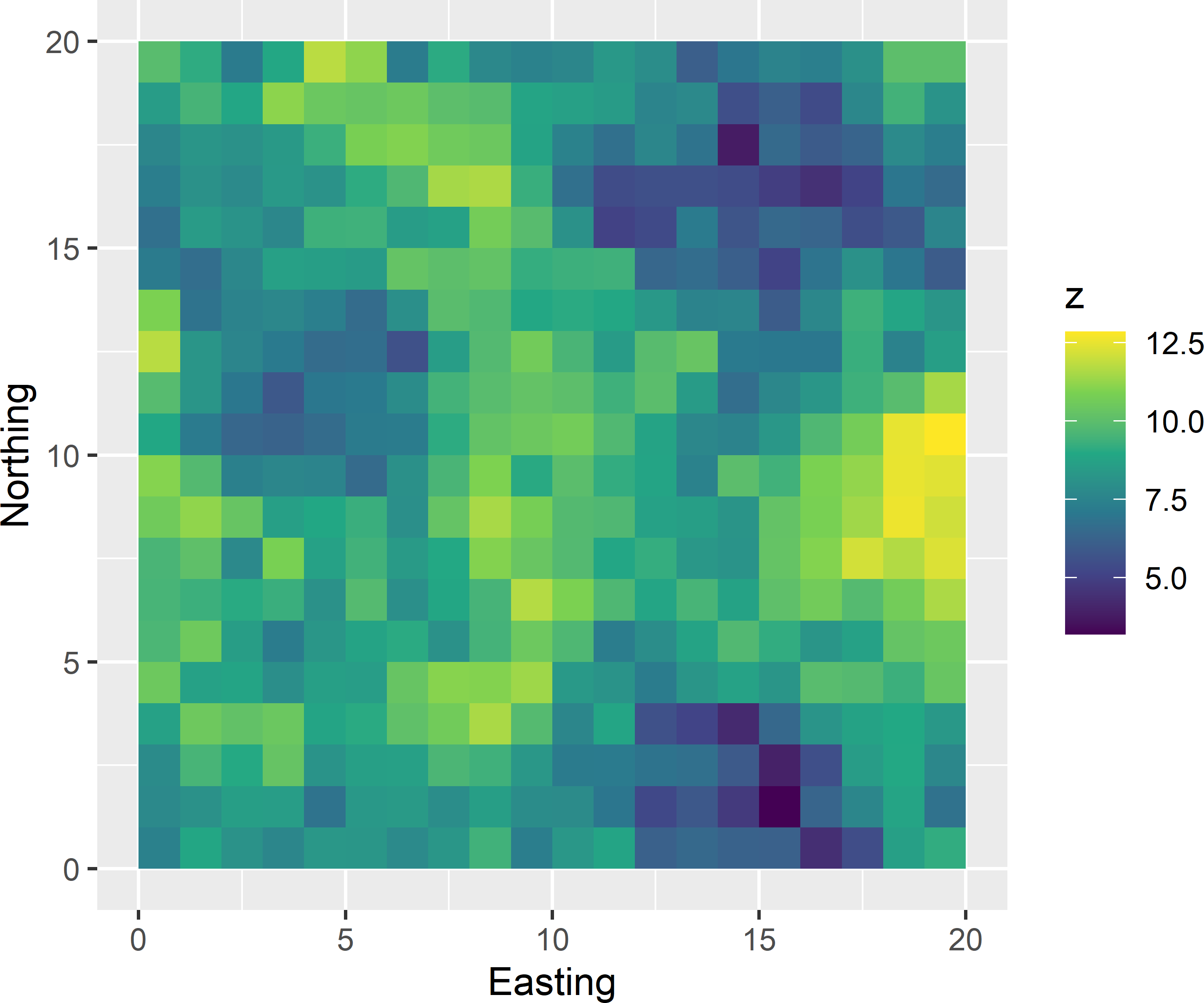
Figure 9.7: Simulated population used for illustration of two-way stratified random sampling.
As a first step, the inclusion probabilities are added to data.frame mypop with the spatial coordinates and simulated values. To keep it simple, I computed inclusion probabilities equal to 2 divided by the number of population units in a cross-classification stratum. Note that this does not imply that a sample is selected with two units per cross-classification stratum. As we will see later, it is possible that in some cross-classification strata no units are selected at all, while in other cross-classification strata more than two units are selected. In multiway stratified sampling, the marginal stratum sample sizes are controlled. The inclusion probabilities should result in six selected units for all four units of map A and eight selected units for all three units of map B.
mypop <- mypop %>%
    group_by(A, B) %>%
    summarise(N_h = n(), .groups = "drop") %>%
    mutate(pi_h = rep(2, 12) / N_h) %>%
    right_join(mypop, by = c("A", "B"))
The next step is to create the design matrix. Two submatrices are computed, one per stratification. The two submatrices are joined columnwise, using function cbind. The columns are multiplied by the vector with inclusion probabilities.
XA <- model.matrix(~ A - 1, mypop)
XB <- model.matrix(~ B - 1, mypop)
X <- cbind(XA, XB)
X <- sweep(X, MARGIN = 1, mypop$pi_h, `*`)
Matrix \(\mathbf{X}\) can be reduced by one column if in the first column the inclusion probabilities of all population units are inserted. This first column contains no zeroes. Balancing on this variable implies that the total sample size is controlled. Now there is no need anymore to control the sample sizes of all marginal strata. It is sufficient to control the sample sizes of three marginal strata of map A (A2, A3, and A4) and two marginal strata of map B (B2 and B3). Given the total sample size, the sample sizes of map units A1 and B1 then cannot be chosen freely anymore.
[1] "(Intercept)" "AA2"         "AA3"         "AA4"         "BB2"
[6] "BB3" This reduced design matrix is not strictly needed for selecting a multiway stratified sample, but it must be used in estimation. If in estimation, as many balancing variables are used as we have marginal strata, the matrix with the sum of squares of the balancing variables (first sum in Equation (9.5)) cannot be inverted (the matrix is singular), and as a consequence the population regression coefficients cannot be estimated.
Finally, the two-way stratified random sample is selected with function samplecube of package sampling.
sample_ind <- samplecube(X = X, pik = mypop$pi_h, method = 1, comment = FALSE)
units <- which(sample_ind > (1 - eps))
mysample <- mypop[units, ]
Figure 9.8 shows the selected sample.
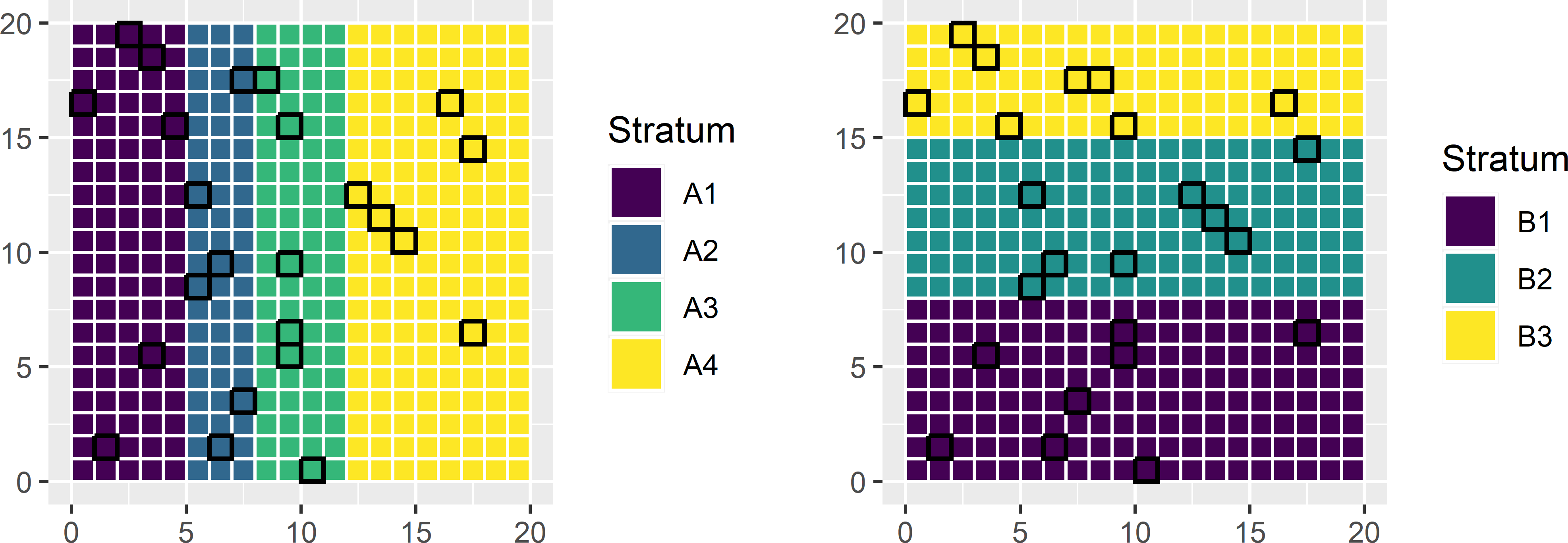
Figure 9.8: Two-way stratified sample.
All marginal stratum sample sizes of map A are six and all marginal stratum sample sizes of map B are eight, as expected. The sample sizes of the cross-classification strata vary from zero to four.
      B1 B2 B3 Sum
  A1   2  0  4   6
  A2   2  3  1   6
  A3   3  1  2   6
  A4   1  4  1   6
  Sum  8  8  8  24
The population mean can be estimated by the \(\pi\) estimator.
[1] 8.688435The variance is estimated as before (Equation (9.3)).
c <- (1 - mysample$pi_h)
b <- estimate_b(
  z = mysample$z / mysample$pi_h, X = X[units, ] / mysample$pi_h, c = c)
zpred <- X %*% b
e <- mysample$z - zpred[units]
n <- nrow(mysample)
v_tz <- n / (n - ncol(X)) * sum(c * (e / mysample$pi_h)^2)
print(v_mz <- v_tz / N^2)
[1] 0.17236889.2 Well-spread sampling
With balanced sampling, the spreading of the sampling units in the space spanned by the balancing variables can be poor. For instance, in Figure 9.1 the Easting coordinates of all units of a sample balanced on Easting can be equal or close to the population mean of 10. So, in this example, balancing does not guarantee a good geographical spreading. Stated more generally, a balanced sample can be selected that shows strong clustering in the space spanned by the balancing variables. This clustering may inflate the standard error of the estimated population total and mean. The clustering in geographical or covariate space can be avoided by the local pivotal method (Grafström, Lundström, and Schelin 2012) and the spatially correlated Poisson sampling method (Grafström 2012).
9.2.1 Local pivotal method
The local pivotal method (LPM) is a modification of the pivotal method explained in Subsection 8.2.2. The only difference with the pivotal method is the selection of the pairs of units. In the pivotal method, at each step two units are selected, for instance, the first two units in the vector with inclusion probabilities after randomising the order of the units. In the local pivotal method, the first unit is selected fully randomly, and the nearest neighbour of this unit is used as its counterpart. Recall that when one unit of a pair is included in the sample, the inclusion probability of its counterpart is decreased. This leads to a better spreading of the sampling units in the space spanned by the spreading variables.
LPM can be used for arbitrary inclusion probabilities. The inclusion probabilities can be equal, but as with the pivotal method these probabilities may also differ among the population units.
Selecting samples with LPM can be done with functions lpm, lpm1, or lpm2 of package BalancedSampling (Grafström and Lisic 2019). Functions lpm1 and lpm2 only differ in the selection of neighbours that are allowed to compete, for details see Grafström, Lundström, and Schelin (2012). For most populations, the two algorithms perform similarly. The algorithm implemented in function lpm is only recommended when the population size is too large for lpm1 or lpm2. It only uses a subset of the population in search for nearest neighbours and is thus not as good. Another function lpm2_kdtree of package SamplingBigData (Lisic and Grafström 2018) is developed for big data sets.
Inclusion probabilities are computed with function inclusionprobabilities of package sampling. A matrix \(\mathbf{X}\) must be defined with the values of the spreading variables of the population units. Figure 9.9 shows a ppswor sample of 40 units selected from the sampling frame of Kandahar, using the spatial coordinates of the population units as spreading variables. Inclusion probabilities are proportional to the agricultural area within the population units. The geographical spreading is improved compared with the sample shown in Figure 8.1.
library(BalancedSampling)
library(sampling)
n <- 40
pi <- inclusionprobabilities(grdKandahar$agri, n)
X <- cbind(grdKandahar$s1, grdKandahar$s2)
set.seed(314)
units <- lpm1(pi, X)
myLPMsample <- grdKandahar[units, ]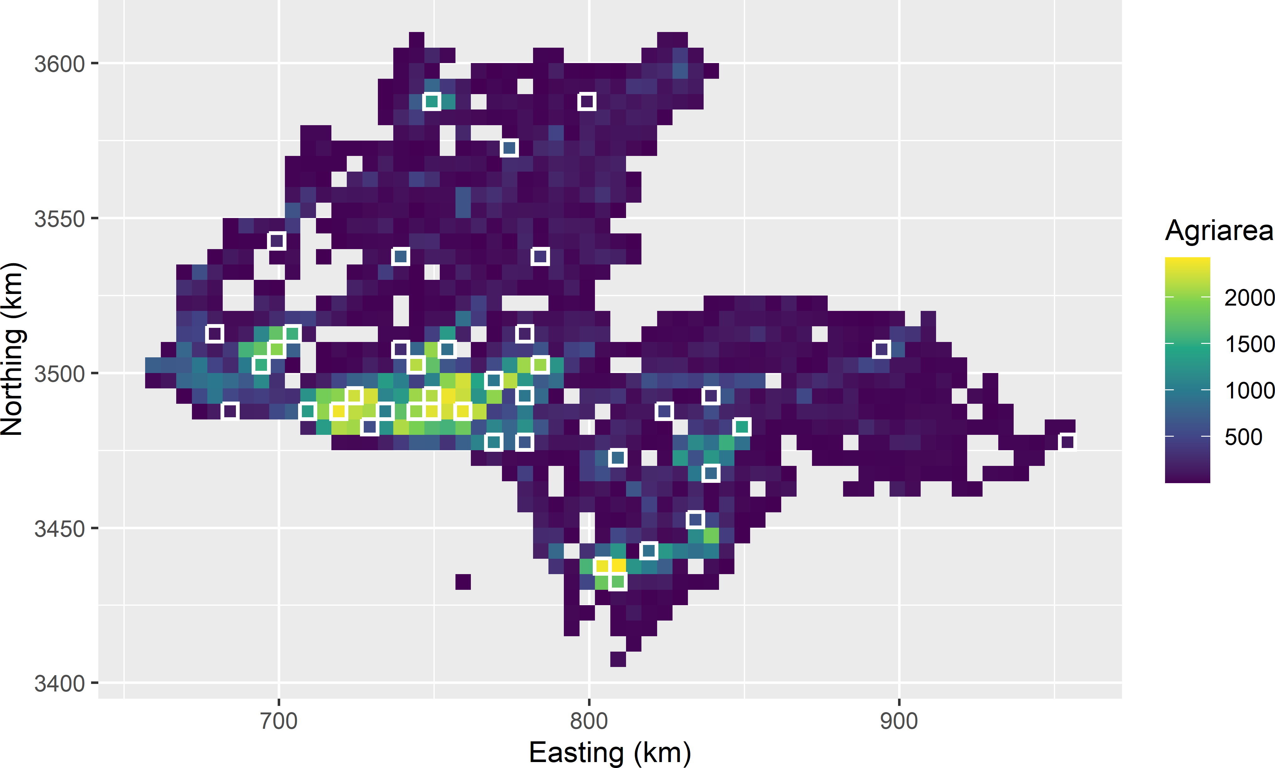
Figure 9.9: Spatial ppswor sample of size 40 from Kandahar, selected by the local pivotal method, using agricultural area as a size variable.
The total poppy area can be estimated with the \(\pi\) estimator (Equation (2.2)).
The estimated total poppy area equals 62,232 ha. The sampling variance of the estimator of the population total with the local pivotal method can be estimated by (Grafström and Schelin 2014)
\[\begin{equation} \widehat{V}(\hat{t}(z)) = \frac{1}{2} \sum_{k \in \mathcal{S}} \left( \frac{z_k}{\pi_k} - \frac{z_{k_j}}{\pi_{k_j}} \right)^2 \;, \tag{9.9} \end{equation}\]
with \({k_j}\) the nearest neighbour of unit \(k\) in the sample. This variance estimator is for the case where we have only one nearest neighbour.
Function vsb of package BalancedSampling is an implementation of a more general variance estimator that accounts for more than one nearest neighbour (equation (6) in Grafström and Schelin (2014)). We expect a somewhat smaller variance compared to pps sampling, so we may use the variance of the pwr estimator (Equation (8.2)) as a conservative variance estimator.
Xsample <- X[units, ]
se_tz_HT <- sqrt(vsb(pi[units], myLPMsample$poppy, Xsample))
pk <- myLPMsample$pi / n
se_tz_pwr <- sqrt(var(myLPMsample$poppy / pk) / n)
The standard error obtained with function vsb equals 12,850 ha, the standard error of the pwr estimator equals 14,094 ha.
As explained above, the LPM design can also be used to select a probability sample well-spread in the space spanned by one or more quantitative covariates. Matrix \(\mathbf{X}\) then should contain the values of the scaled (standardised) covariates instead of the spatial coordinates.
Exercises
- Geographical spreading of the sampling units can also be achieved by random sampling from compact geographical strata (geostrata) (Section 4.6). Can you think of one or more advantages of LPM sampling over random sampling from geostrata?
9.2.2 Generalised random-tessellation stratified sampling
Generalised random-tessellation stratified (GRTS) sampling is designed for sampling discrete objects scattered throughout space, think for instance of the lakes in Finland, segments of hedgerows in England, etc. Each object is represented by a point in 2D-space. It is a complicated design, and for sampling points from a continuous universe or raster cells from a finite population, I recommend more simple designs such as the local pivotal method (Subsection 9.2.1), balanced sampling with geographical spreading (Section 9.3), or sampling from compact geographical strata (Section 4.6). Let me try to explain the GRTS design with a simple example of a finite population of point objects in a circular study area (Figure 9.10). For a more detailed description of this design, refer to Hankin, Mohr, and Newman (2019). As a first step, a square bounding box of the study area is constructed. This bounding box is recursively partitioned into square grid cells. First, 2 \(\times\) 2 grid cells are constructed. These grid cells are numbered in a predefined order. In Figure 9.10 this numbering is from lower left, lower right, upper left to upper right. Each grid cell is then subdivided into four subcells; the subcells are numbered using the same order. This is repeated until at most one population unit occurs in each subcell. For our population only two iterations were needed, leading to 4 \(\times\) 4 subcells. Note that two subcells are empty. Each address of a subcell consists of two digits: the first digit refers to the grid cell, the second digit to the subcell.
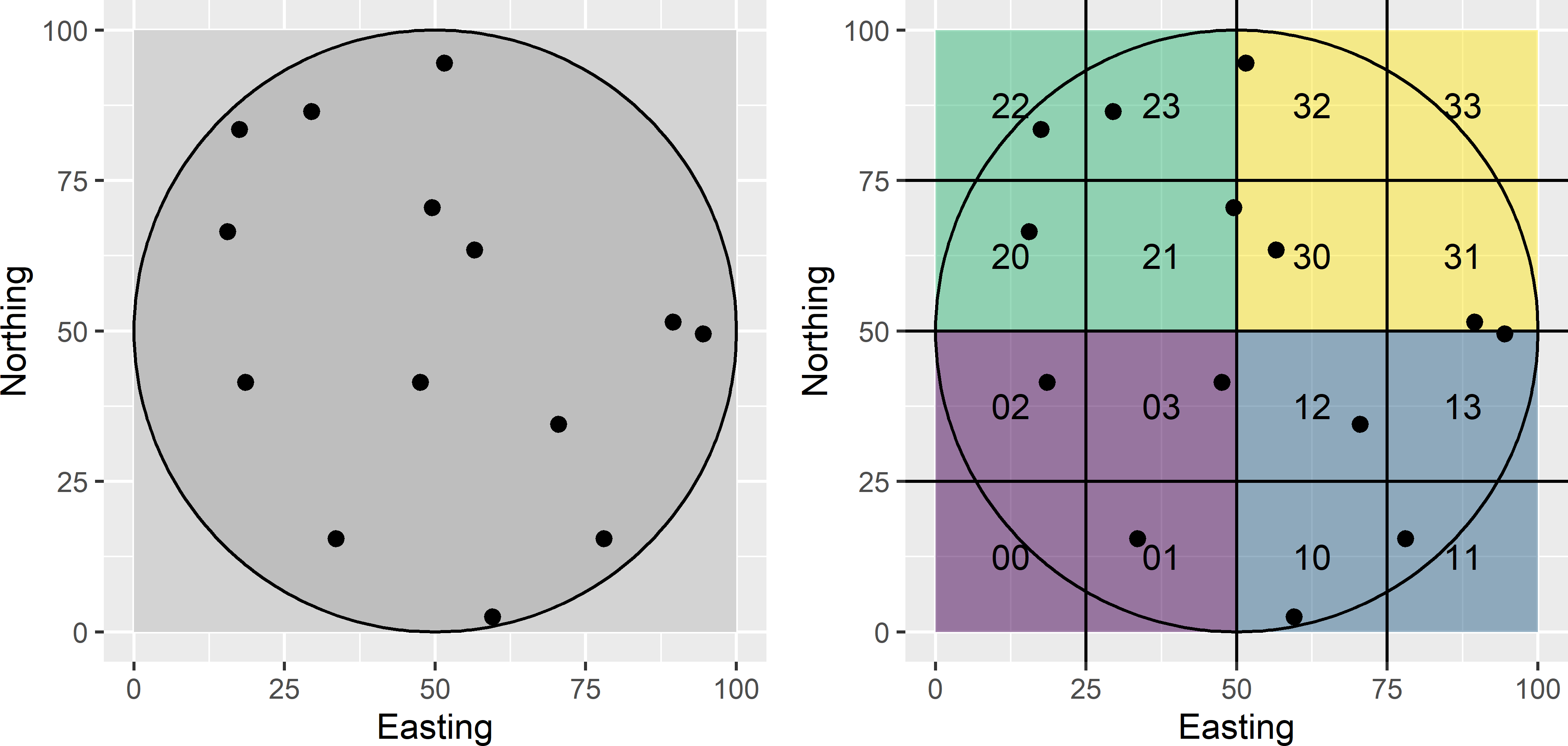
Figure 9.10: Numbering of grid cells and subcells for GRTS sampling.
The next step is to place the 16 subcells on a line in a random order. The randomisation is done hierarchically. First, the four grid cells at the highest level are randomised. In our example, the randomised order is 1, 2, 3, 0 (Figure 9.11). Next, within each grid cell, the order of the subcells is randomised. This is done independently for the grid cells. In our example, for grid cell 1 the randomised order of the subcells is 2, 1, 3, 0 (Figure 9.11). Note that the empty subcells (0,0) and (3,3) are removed from the line.
set.seed(314)
ord <- sample(4, 4)
myfinpop_rand <- NULL
for (i in ord) {
  units <- which(myfinpop$partit1 == i)
  units_rand <- sample(units, size = length(units))
  myfinpop_rand <- rbind(myfinpop_rand, myfinpop[units_rand, ])
}
After the subcells have been placed on a line, a one-dimensional systematic random sample is selected (Figure 9.11), see also Subsection 8.2.1. This can be done either with equal or unequal inclusion probabilities. With equal inclusion probabilities, the length of the intervals representing the population units is constant. With unequal inclusion probabilities, the interval lengths are proportional to a size variable. For a sample size of \(n\), the total line is divided into \(n\) segments of equal length. A random point is selected in the first segment, and the other points of the systematic sample are determined. Finally, the population units corresponding to the selected systematic sample are identified. With equal probabilities, the five selected units are the units in subcells 11, 23, 22, 32, and 03 (Figure 9.11).
size <- rep(1, N)
n <- 5
interval <- sum(size) / n
start <- round(runif(1) * interval, 2)
mysys <- c(start, 1:(n - 1) * interval + start)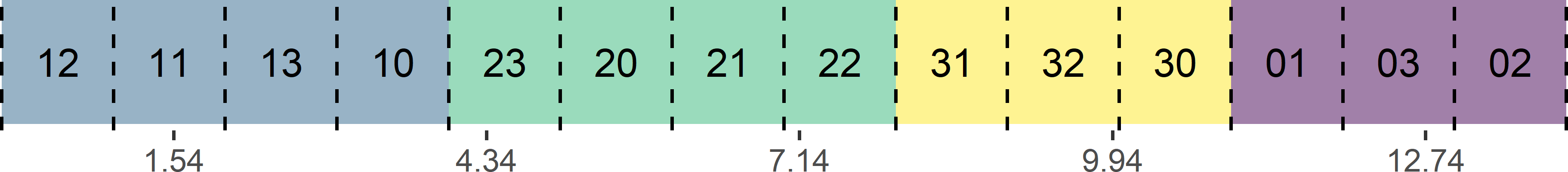
Figure 9.11: Systematic random sample along a line with equal inclusion probabilities.
Figure 9.12 shows a systematic random sample along a line with unequal inclusion probabilities. The inclusion probabilities are proportional to a size variable, with values 1, 2, 3, or 4. The selected population units are the units in subcells 10, 20, 31, 01, and 02.
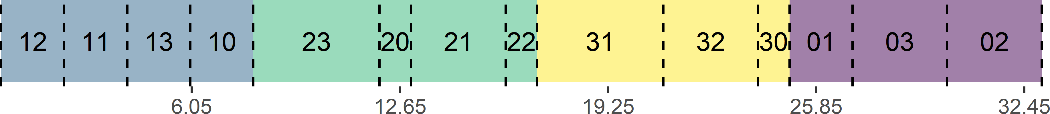
Figure 9.12: Systematic random sample along a line with inclusion probabilities proportional to size.
GRTS samples can be selected with function grts of package spsurvey (Dumelle et al. 2021). The next code chunk shows the selection of a GRTS sample of 40 units from Kandahar. Tibble grdKandahar is first converted to an sf object with function st_as_sf of package sf (E. Pebesma 2018). The data set is using a UTM projection (zone 41N) with WGS84 datum. This projection is passed to function st_as_df with argument crs (crs = 32641). Argument sframe of function grts specifies the sampling frame. The sample size is passed to function grts with argument n_base. Argument seltype is set to proportional to select units with probabilities proportional to an ancillary variable which is passed to function grts with argument aux_var.
library(spsurvey)
library(sf)
sframe_sf <- st_as_sf(grdKandahar, coords = c("s1", "s2"), crs = 32641)
set.seed(314)
res <- grts(
  sframe = sframe_sf, n_base = 40, seltype = "proportional", aux_var = "agri")
myGRTSsample <- res$sites_base
Function cont_analysis computes the ratio estimator of the population mean and its standard error. The estimated mean is multiplied by the total number of population units to obtain a ratio estimate of the population total.
myGRTSsample$siteID <- paste0("siteID", seq_len(nrow(myGRTSsample)))
res <- cont_analysis(myGRTSsample,
       vars = "poppy", siteID = "siteID", weight = "wgt", statistics = "Mean")
tz_ratio <- res$Mean$Estimate * nrow(grdKandahar)
se_tz_ratio <- res$Mean$StdError * nrow(grdKandahar)
The estimated total poppy area is 109,809 ha, and the estimated standard error is 24,327 ha.
The alternative is to estimate the total poppy area by the \(\pi\) estimator. Function vsb of package BalancedSampling can be used to estimate the standard error of the \(\pi\) estimator.
tz_HT <- sum(myGRTSsample$poppy / myGRTSsample$ip)
Xsample <- st_coordinates(myGRTSsample)
se_tz_HT <- sqrt(vsb(myGRTSsample$ip, myGRTSsample$poppy, Xsample))
The estimated total is 71,634 ha, and the estimated standard error is 12,593 ha.
9.3 Balanced sampling with spreading
As mentioned in the introduction to this chapter, a sample balanced on a covariate still may have a poor spreading along the axis spanned by the covariate. Grafström and Tillé (2013) presented a method for selecting balanced samples that are also well-spread in the space spanned by the covariates, which they refer to as doubly balanced sampling. If we take one or more covariates as balancing variables and, besides, Easting and Northing as spreading variables, this leads to balanced samples with good geographical spreading. When the residuals of the regression model show spatial structure (are spatially correlated), the estimated population mean of the study variable becomes more precise thanks to the improved geographical spreading. Balanced samples with spreading can be selected with function lcube of package BalancedSampling. This is illustrated with Eastern Amazonia, using as before lnSWIR2 for balancing the sample.
library(BalancedSampling)
N <- nrow(grdAmazonia)
n <- 100
Xbal <- cbind(rep(1, times = N), grdAmazonia$lnSWIR2)
Xspread <- cbind(grdAmazonia$x1, grdAmazonia$x2)
pi <- rep(n / N, times = N)
set.seed(314)
units <- lcube(Xbal = Xbal, Xspread = Xspread, prob = pi)
mysample <- grdAmazonia[units, ]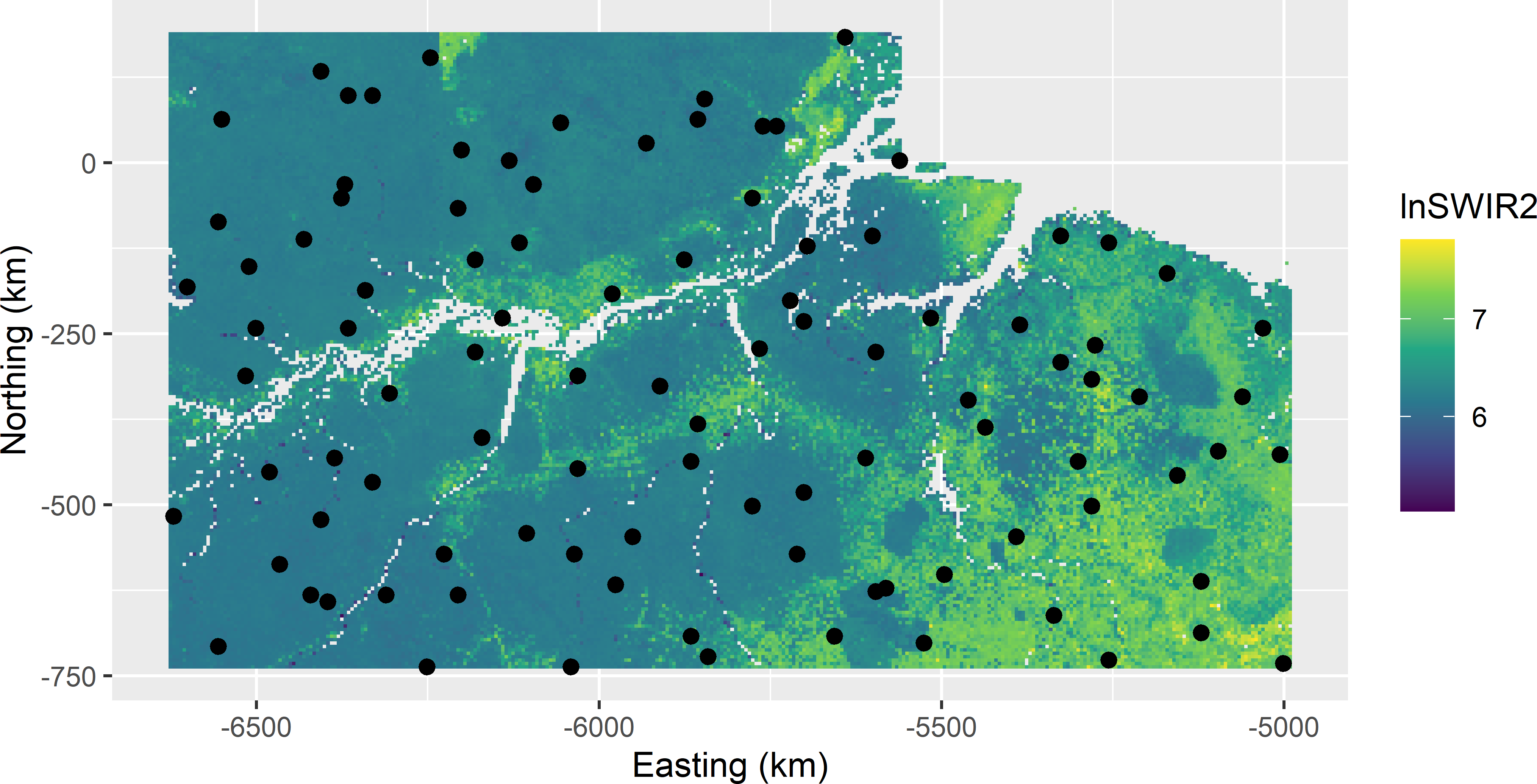
Figure 9.13: Sample balanced on lnSWIR2 with geographical spreading from Eastern Amazonia.
The selected sample is shown in Figure 9.13. Comparing this sample with the balanced sample of Figure 9.3 shows that the geographical spreading of the sample is improved, although there still are some close points. I used equal inclusion probabilities, so the \(\pi\) estimate of the mean is equal to the sample mean, which is equal to 225.6 109 kg ha-1.
The variance of the \(\pi\) estimator of the mean can be estimated by (equation (7) of Grafström and Tillé (2013))
\[\begin{equation} \widehat{V}(\hat{\bar{z}}) = \frac{n}{n-p}\frac{p}{p+1} \sum_{k \in \mathcal{S}}(1-\pi_k) \left(\frac{e_k}{\pi_k}-\bar{e}_k \right)^2 \;, \tag{9.10} \end{equation}\]
with \(p\) the number of balancing variables, \(e_k\) the regression model residual of unit \(k\) (Equation (9.4)), and \(\bar{e}_k\) the local mean of the residuals of this unit, computed by
\[\begin{equation} \bar{e}_k = \frac{\sum_{j=1}^{p+1}(1-\pi_j)\frac{e_j}{\pi_j}}{\sum_{j=1}^{p+1}(1-\pi_j)}\;. \tag{9.11} \end{equation}\]
The variance estimator can be computed with functions localmean_weight and localmean_var of package spsurvey (Dumelle et al. 2021).
library(spsurvey)
pi <- rep(n / N, n)
c <- (1 - pi)
b <- estimate_b(z = mysample$AGB / pi, X = Xbal[units, ] / pi, c = c)
zpred <- Xbal %*% b
e <- mysample$AGB - zpred[units]
weights <- localmean_weight(x = mysample$x1, y = mysample$x2, prb = pi, nbh = 3)
v_mz <- localmean_var(z = e / pi, weight_1st = weights) / N^2
The estimated standard error is 2.8 109 kg ha-1, which is considerably smaller than the estimated standard error of the balanced sample without geographical spreading.