Two-stage cluster random sampling
As opposed to cluster random sampling in which all population units of a cluster are observed (Chapter 6), in two-stage cluster random sampling not all units of the selected clusters are observed, but only some. In two-stage cluster random sampling the clusters will generally be contiguous groups of units, for instance all points in a map polygon (the polygons on the map are the clusters), whereas in one-stage cluster random sampling the clusters generally are non-contiguous. The units to be observed are selected by random subsampling of the randomly selected clusters. In two-stage cluster sampling, the clusters are commonly referred to as primary sampling units (PSUs) and the units selected in the second stage as the secondary sampling units (SSUs).
As with cluster random sampling, two-stage cluster random sampling may lead to a strong spatial clustering of the selected population units in the study area. This may save considerable time for fieldwork, and more population units can be observed for the same budget. However, due to the spatial clustering the estimates will generally be less precise compared to samples of the same size selected by a design that leads to a much better spreading of the sampling units throughout the study area, such as systematic random sampling.
In two-stage cluster random sampling, in principle any type of sampling design can be used at the two stages, leading to numerous combinations. An example is (SI,SI), in which both PSUs and SSUs are selected by simple random sampling.
Commonly, the PSUs have unequal size, i.e., the number of SSUs (finite population) or the area (infinite population) are not equal for all PSUs. Think for instance of the agricultural fields, forest stands, lakes, river sections, etc. in an area. If the PSUs are of unequal size, then PSUs can best be selected with probabilities proportional to their size (pps). Recall that in (one-stage) cluster random sampling, I also recommended to select the clusters with probabilities proportional to their size, see Chapter 6. If the total of the study variable of a PSU is proportional to its size, then pps sampling leads to more precise estimates compared to simple random sampling of PSUs. Also, with pps sampling of PSUs, the estimation of means or totals and of their sampling variances is much simpler compared to selection with equal probabilities. Implementation of selection with probabilities proportional to size is easiest when units are replaced (pps with replacement, ppswr). This implies that a PSU might be selected more than once, especially if the total number of PSUs in the population is small compared to the number of PSU draws (large sampling fraction in first stage).
Using a list as a sampling frame, the following algorithm can be used to select \(n\) times a PSU by ppswr from a total of \(N\) PSUs in the population:
- Select randomly one SSU from the list with \(M=\sum_{j=1}^N M_j\) SSUs (\(M_j\) is the number of SSUs of PSU \(j\)), and determine the PSU of the selected SSU.
- Repeat step 1 until \(n\) selections have been made.
In the first stage, an SSU is selected in order to select a PSU. This may seem unnecessarily complicated. The reason for this is that this procedure automatically adjusts for the size of the PSUs (number of SSUs within a PSU), i.e., a PSU is selected with probability proportional to its size. In the second stage, a pre-determined number of SSUs, \(m_{j}\), is selected every time PSU \(j\) is selected.
Note that the SSU selected in the first step of the two algorithms primarily serves to identify the PSU, but these SSUs can also be used as selected SSUs.
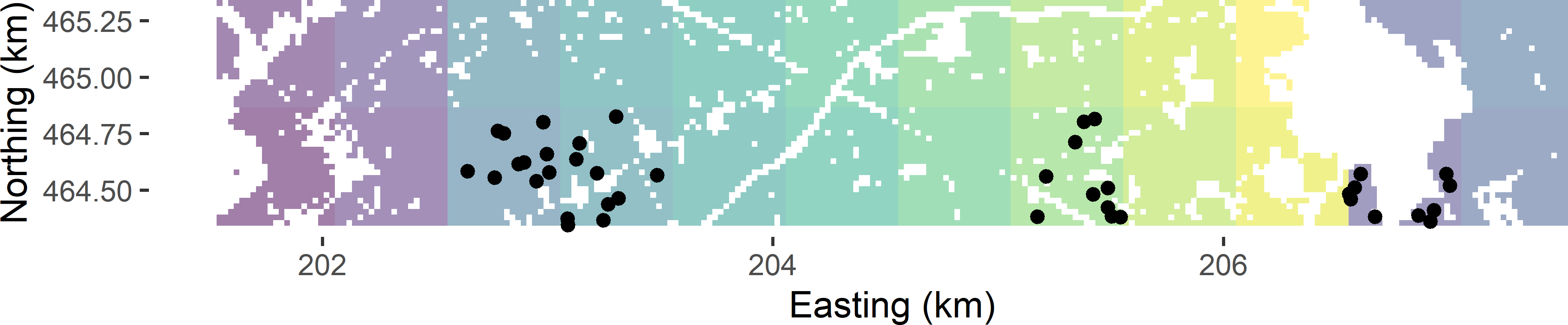
The selection of a two-stage cluster random sample is illustrated again with Voorst. Twenty-four 0.5 km squares are constructed that serve as PSUs.
Due to built-up areas, roads, etc., the PSUs in Voorst have unequal size, i.e., the number of SSUs (points, in our case) within the PSUs varies among the PSUs.
cell_size <- 25
w <- 500 #width of zones
grdVoorst <- grdVoorst %>%
    mutate(zone_s1 = s1 %>% findInterval(min(s1) + 1:11 * w + 0.5 * cell_size),
           zone_s2  = s2 %>% findInterval(min(s2) + w + 0.5 * cell_size),
           psu = str_c(zone_s1, zone_s2, sep = "_"))
In the next code chunk, a function is defined to select a two-stage cluster random sample from an infinite population, discretised by a finite number of points, being the centres of grid cells.
twostage <- function(sframe, psu, n, m) {
  units <- sample(nrow(sframe), size = n, replace = TRUE)
  mypsusample <- sframe$psu[units]
  ssunits <- NULL
  for (i in seq_len(length(mypsusample))) {
    ssunit <- sample(
      x = which(sframe$psu == mypsusample[i]), size = m, replace = TRUE)
    ssunits <- c(ssunits, ssunit)
  }
  psudraw <- rep(c(1:n), each = m)
  mysample <- data.frame(ssunits, sframe[ssunits, ], psudraw)
  mysample
}
Note that both the PSUs and the SSUs are selected with replacement. If a grid cell centre is selected, one point is selected fully randomly from that grid cell. This is done by shifting the centre of the grid cell to a random point within the selected grid cell with function jitter, see code chunk hereafter. In every grid cell, there is an infinite number of points, so we must select the grid cell centres with replacement. If a grid cell is selected more than once, more than one point is selected from the associated grid cell. Column psudraw in the output data frame of function twostage is needed in estimation because PSUs are selected with replacement. In case a PSU is selected more than once, multiple estimates of the mean of that PSU are used in estimation, see next section.
In the next code chunk, function twostage is used to select four times a PSU (\(n=4\)), with probabilities proportional to size and with replacement (ppswr). The second stage sample size equals 10 for all PSUs (\(m_j=10,\; j = 1, \dots, N\)). These SSUs are selected by simple random sampling.
n <- 4
m <- 10
cell_size <- 25
set.seed(314)
mysample <- grdVoorst %>%
  twostage(psu = "psu", n = n, m = m) %>%
  mutate(s1 = s1 %>% jitter(amount = cell_size / 2),
         s2 = s2 %>% jitter(amount = cell_size / 2))
Figure 7.1 shows the selected sample.
Estimation of population parameters
The population total can be estimated by substituting the estimated cluster (PSU) totals in Equation (6.4). This yields the following estimator for the population total:
\[\begin{equation}
\hat{t}(z) = \frac{M}{n} \sum_{j \in \mathcal{S}} \frac{\hat{t}_{j}(z)}{M_{j}} = \frac{M}{n} \sum_{j \in \mathcal{S}} \hat{\bar{z}}_{j} \;,
\tag{7.1}
\end{equation}\]
where \(n\) is the number of PSU selections and \(M_{j}\) is the total number of SSUs in PSU \(j\). This shows that the mean of cluster \(j\), \(\bar{z}_j\), is replaced by the estimated mean of PSU \(j\), \(\hat{\bar{z}}_j\). Dividing this estimator by the total number of population units \(M\) gives the pwr estimator of the population mean:
\[\begin{equation}
\hat{\bar{\bar{z}}}=
\frac{1}{n}\sum\limits_{j \in \mathcal{S}}\hat{\bar{z}}_{j} \;,
\tag{7.2}
\end{equation}\]
with \(\hat{\bar{z}}_{j}\) the estimated mean of the PSU \(j\). With simple random sampling of SSUs, this mean can be estimated by the sample mean of this PSU. Note the two bars in \(\hat{\bar{\bar{z}}}\), indicating that the population mean is estimated as the mean of estimated PSU means. When \(m_j\) is equal for all PSUs, the sampling design is self-weighting, i.e., the average of \(z\) over all selected SSUs is an unbiased estimator of the population mean.
For an infinite population of points, the population total is estimated by multiplying the estimated population mean (Equation (7.2)) by the area of the study area.
The sampling variance of the estimator of the mean with two-stage cluster random sampling, PSUs selected with probabilities proportional to size with replacement, SSUs selected by simple random sampling, with replacement in case of finite populations, and \(m_j = m, \; j = 1, \dots, N\), is equal to (Cochran (1977), equation (11.33))
\[\begin{equation}
V(\hat{\bar{\bar{z}}}) = \frac{S^2_{\mathrm{b}}}{n} + \frac{S^2_{\mathrm{w}}}{n\;m} \;,
\tag{7.3}
\end{equation}\]
with
\[\begin{equation}
S^2_{\mathrm{b}}=\sum_{j=1}^N p_j\left(\bar{z}_j-\bar{z}\right)^2
\tag{7.4}
\end{equation}\]
and
\[\begin{equation}
S^2_{\mathrm{w}}=\sum_{j=1}^N p_j S^2_j \;,
\tag{7.5}
\end{equation}\]
with \(N\) the total number of PSUs in the population, \(p_j=M_j/M\) the draw-by-draw selection probability of PSU \(j\), \(\bar{z}_j\) the mean of PSU \(j\), \(\bar{z}\) the population mean of \(z\), and \(S^2_j\) the variance of \(z\) within PSU \(j\):
\[\begin{equation}
S^2_j = \frac{1}{M_j} \sum_{k=1}^{M_j} (z_{kj}-\bar{z}_j)^2 \;.
\tag{7.6}
\end{equation}\]
The first term of Equation
(7.3) is equal to the variance of Equation
(6.6). This variance component accounts for the variance of the true PSU means within the population. The second variance component quantifies our additional uncertainty about the population mean, as we do not observe all SSUs of the selected PSUs, but only a subset (sample) of these units.
The sampling variance of the estimator of the population mean can simply be estimated by
\[\begin{equation}
\widehat{V}\!\left(\hat{\bar{\bar{z}}}\right)=\frac{\widehat{S^2}(\hat{\bar{z}})}{n} \;,
\tag{7.7}
\end{equation}\]
with \(\widehat{S^2}(\hat{\bar{z}})\) the estimated variance of the estimated PSU means:
\[\begin{equation}
\widehat{S^2}(\hat{\bar{z}}) = \frac{1}{n-1}\sum_{j \in \mathcal{S}}(\hat{\bar{z}}_{j}-\hat{\bar{\bar{z}}})^2 \;,
\tag{7.8}
\end{equation}\]
with \(\hat{\bar{z}}_{j}\) the estimated mean of PSU \(j\) and \(\hat{\bar{\bar{z}}}\) the estimated population mean (Equation (7.2)).
Neither the sizes of the PSUs,
\(M_j\), nor the secondary sample sizes
\(m_{j}\) occur in Equations
(7.7) and
(7.8). This simplicity is due to the fact that the PSUs are selected with replacement and with probabilities proportional to their size. The effect of the secondary sample sizes on the variance is implicitly accounted for. To understand this, note that the larger
\(m_{j}\), the less variable
\(\hat{\bar{z}}_{j}\), and the smaller its contribution to the variance.
Let us assume a linear model for the total costs: \(C = c_0 + c_1n + c_2nm\), with \(c_0\) the fixed costs, \(c_1\) the costs per PSU, and \(c_2\) the costs per SSU. We want to minimise the total costs, under the constraint that the variance of the estimator of the population mean may not exceed \(V_{\mathrm{max}}\). The total costs can then be minimised by selecting (de Gruijter et al. 2006)
\[\begin{equation}
n=\frac{1}{V_{\mathrm{max}}}\left(S_{\mathrm{w}}S_{\mathrm{b}}\sqrt{\frac{c_2}{c_1}}+S^2_{\mathrm{b}}\right)
\tag{7.9}
\end{equation}\]
PSUs and
\[\begin{equation}
m=\frac{S_{\mathrm{w}}}{S_{\mathrm{b}}}\sqrt{\frac{c_1}{c_2}}
\tag{7.10}
\end{equation}\]
SSUs per PSU.
Conversely, given a budget \(C_{\mathrm{max}}\), the optimal number of PSU selections can be computed with (de Gruijter et al. 2006)
\[\begin{equation}
n=\frac{C_{\mathrm{max}}S_{\mathrm{b}}}{S_{\mathrm{w}}\sqrt{c_1c_2}+S_{\mathrm{b}}c_1}\;,
\tag{7.11}
\end{equation}\]
and \(m\) as above.
In R the population mean and the sampling variance of the estimator of the mean can be estimated as follows.
est <- mysample %>%
  group_by(psudraw) %>%
  summarise(mz_psu = mean(z)) %>%
  summarise(mz = mean(mz_psu),
            se_mz = sqrt(var(mz_psu) / n()))
The estimated mean equals 71.2 g kg-1, and the estimated standard error equals 18.6 g kg-1. The sampling design is self-weighting, and so the estimated mean is equal to the sample mean.
[1] 71.18013
The same estimate is obtained with functions svydesign and svymean of package survey (Lumley 2021). The estimator of the population total can be written as a weighted sum of the observations with all weights equal to \(M/(n\;m)\). These weights are passed to function svydesign with argument weight.
library(survey)
M <- nrow(grdVoorst)
mysample$weights <- M / (n * m)
design_2stage <- svydesign(
  id = ~ psudraw, weight = ~ weights, data = mysample)
svymean(~ z, design_2stage, deff = "replace")
    mean     SE   DEff
z 71.180 18.563 4.2985
Similar to (one-stage) cluster random sampling, the estimated design effect is much larger than 1.
A confidence interval estimate of the population mean can be computed with method confint. The number of degrees of freedom equals the number of PSU draws minus 1.
confint(svymean(~ z, design_2stage, df = degf(design_2stage), level = 0.95))
     2.5 %  97.5 %
z 34.79724 107.563
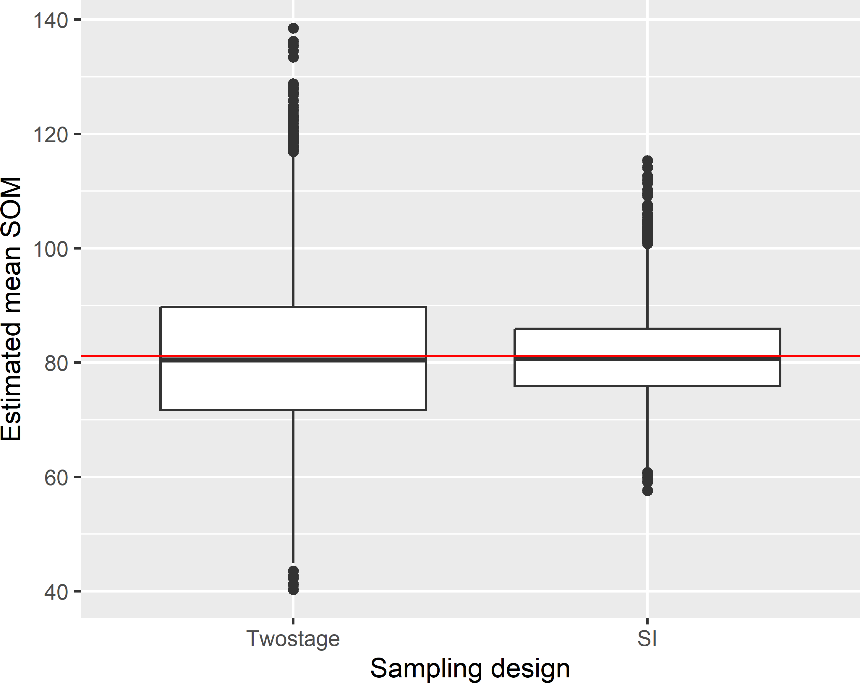
Figure 7.2 shows the approximated sampling distribution of the pwr estimator of the mean soil organic matter (SOM) concentration with two-stage cluster random sampling and of the \(\pi\) estimator with simple random sampling from Voorst, obtained by repeating the random sampling with each design and estimation 10,000 times. For simple random sampling the sample size is equal to \(n \times m\).
The variance of the 10,000 means with two-stage cluster random sampling equals 179.6 (g kg-1)2. This is considerably larger than with simple random sampling: 56.3 (g kg-1)2. The average of the estimated variances with two-stage cluster random sampling equals 182.5 (g kg-1)2.
Optimal sample sizes for two-stage cluster random sampling (ppswr in first stage, simple random sampling without replacement in second stage) can be computed with function clusOpt2 of R package PracTools (Valliant, Dever, and Kreuter (2021), Valliant, Dever, and Kreuter (2018)). This function requires as input various variance measures, which can be computed with function BW2stagePPS, in case the study variable is known for the whole population or estimated from a sample with function BW2stagePPSe. This is left as an exercise (Exercise 5).
Exercises
- Write an R script to compute for Voorst the true sampling variance of the estimator of the mean SOM concentration for two-stage cluster random sampling, PSUs selected by ppswr, \(n=4\), and \(m=10\), see Equation (7.3).
- Do you expect that the standard error of the estimator of the population mean with ten PSU draws (\(n=10\)) and four SSUs per PSU draw (\(m=4\)) is larger or smaller than with four PSU draws (\(n=4\)) and ten SSUs per PSU draw (\(m=10\))?
- Compute the optimal sample sizes \(n\) and \(m\) for a maximum variance of the estimator of the mean SOM concentration of 1, \(c_1=2\) monetary units, and \(c_2=1\) monetary unit, see Equations (7.9) and (7.10).
- Compute the optimal sample sizes \(n\) and \(m\) for a budget of 100 monetary units, \(c_1=2\) monetary units, and \(c_2=1\) monetary unit, see Equations (7.11) and (7.10).
- Use function
clusOpt2 of R package PracTools to compute optimal sample sizes given the precision requirement for the estimated population mean of Exercise 3 and given the budget of Exercise 4. Use function BW2stagePPS to compute the variance measures needed as input for function clusOpt2. Note that the precision requirement of function clusOpt2 is the coefficient of variation of the estimated population total, i.e., the standard deviation of the estimated population total divided by the population total. Compute this coefficient of variation from the maximum variance of the estimator of the population mean used in Exercise 3.
- The variance of the estimator for the population total is (Cochran 1977):
\[\begin{equation}
V(\hat{t}(z)) = \frac{1}{n} \sum_{j=1}^N p_j\left(\frac{t_j(z)}{p_j}-t(z)\right)^2 + \frac{1}{n} \sum_{j=1}^N \frac{M_j^2 (1-f_{2j})S^2_j}{m_j p_j} \;,
\tag{7.12}
\end{equation}\]
with \(\hat{t}(z)\) and \(t(z)\) the estimated and the true population total of \(z\), respectively, \(t_j(z)\) the total of PSU \(j\), and \(p_j = M_j/M\). Use \(m_j = m, \;j = 1, \dots, N\), and \(f_{2j}=0\), i.e., sampling from infinite population, or sampling of SSUs within PSUs by simple random sampling with replacement from finite population. Derive the variance of the estimator for the population mean, Equation (7.3), from Equation (7.12).
Primary sampling units selected without replacement
Similar to cluster random sampling, we may prefer to select the PSUs without replacement. This leads to less strong spatial clustering of the sampling points, especially with large sampling fractions of PSUs. Sampling without replacement of PSUs can be done with function UPpivotal of package sampling (Tillé and Matei 2021), see Subsection 8.2.2. The second stage sample of SSUs is selected with function strata of the same package, using the PSUs as strata.
library(sampling)
M_psu <- tapply(grdVoorst$z, INDEX = grdVoorst$psu, FUN = length)
n <- 6; m <- 10
pi <- inclusionprobabilities(M_psu, n)
set.seed(314)
sampleind <- UPpivotal(pik = pi, eps = 1e-6)
psus <- sort(unique(grdVoorst$psu))
sampledpsus <- psus[sampleind == 1]
mysample_stage1 <- grdVoorst[grdVoorst$psu %in% sampledpsus, ]
units <- sampling::strata(mysample_stage1, stratanames = "psu",
  size = rep(m, n), method = "srswor")
mysample <- getdata(mysample_stage1, units)
mysample$ssunits <- units$ID_unit
mysample$pi <- n * m / M
print(mean_HT <- sum(mysample$z / mysample$pi) / M)
[1] 100.039
The population mean can be estimated with function svymean of package survey. To estimate the variance, a simple solution is to treat the two-stage cluster random sample as a pps sample with replacement, so that variance can be estimated with Equation (7.7). With small sampling fractions of PSUs, the overestimation of the variance is negligible. With larger sampling fractions, Brewer’s method is recommended, see Berger (2004) (option 2).
mysample$fpc1 <- n * M_psu[mysample$psu] / M
mysample$fpc2 <- m / M_psu[mysample$psu]
design_2stageppswor <- svydesign(id = ~ psu + ssunits, data = mysample,
  pps = "brewer", fpc = ~ fpc1 + fpc2)
svymean(~ z, design_2stageppswor)
    mean     SE
z 100.04 19.883
Simple random sampling of primary sampling units
Suppose the PSUs are for some reason not selected with probabilities proportional to their size, but by simple random sampling without replacement. The inclusion probabilities of the PSUs then equal \(\pi_j=n/N,\; j = 1, \dots, N\), and the population total can be estimated by (compare with Equation (6.9))
\[\begin{equation}
\hat{t}(z) = \sum_{j=1}^n \frac{\hat{t}_j(z)}{\pi_j} = \frac{N}{n} \sum_{j=1}^n \hat{t}_j(z)\;,
\tag{7.13}
\end{equation}\]
with \(\hat{t}_j(z)\) an estimator of the total of PSU \(j\). The population mean can be estimated by dividing this estimator by the population size \(M\).
Alternatively, we may estimate the population mean by dividing the estimate of the population total by the estimated population size. The population size can be estimated by the \(\pi\) estimator, see Equation (6.11). The \(\pi\) estimator and the ratio estimator are equal when the PSUs are selected by ppswr, but not so when the PSUs of different size are selected with equal probabilities. This is shown below. First, a sample is selected by selecting both PSUs and SSUs by simple random sampling without replacement.
library(sampling)
set.seed(314)
psus <- sort(unique(grdVoorst$psu))
ids_psu <- sample(length(psus), size = n, replace = FALSE)
sampledpsus <- psus[ids_psu]
mysample_stage1 <- grdVoorst[grdVoorst$psu %in% sampledpsus, ]
units <- sampling::strata(mysample_stage1, stratanames = "psu",
  size = rep(m, n), method = "srswor")
mysample <- getdata(mysample_stage1, units)
mysample$ssunits <- units$ID_unit
The population mean is estimated by the \(\pi\) estimator and the ratio estimator.
N <- length(unique(grdVoorst$psu))
M_psu <- tapply(grdVoorst$z, INDEX = grdVoorst$psu, FUN = length)
pi_psu <- n / N
pi_ssu <- m / M_psu[mysample$psu]
est <- mysample %>%
  mutate(pi = pi_psu * pi_ssu,
         z_piexpanded = z / pi) %>%
  summarise(tz_HT = sum(z_piexpanded),
            mz_HT = tz_HT / M,
            M_HT = sum(1 / pi),
            mz_ratio = tz_HT / M_HT)
The \(\pi\) estimate equals 79.0 g kg-1, and the ratio estimate equals 79.8 g kg-1. The \(\pi\) estimate of the population mean can also be computed by first estimating totals of PSUs, see Equation (7.13).
tz_psu <- tapply(mysample$z / pi_ssu, INDEX = mysample$psu, FUN = sum)
tz_HT <- sum(tz_psu / pi_psu)
(mz_HT <- tz_HT / M)
[1] 78.99646
The variance of the \(\pi\) estimator of the population mean can be estimated by first estimating the variance of the estimator of the PSU totals:
\[\begin{equation}
\widehat{V}(\hat{t}(z)) = N^2\left(1-\frac{n}{N}\right)\frac{\widehat{S^2}(\hat{t}_i(z))}{n} \;,
\tag{7.14}
\end{equation}\]
and dividing this variance by the squared number of population units:
\[\begin{equation}
\widehat{V}(\hat{\bar{\bar{z}}}) = \frac{1}{M^2} \widehat{V}(\hat{t}(z)) \;,
\tag{7.15}
\end{equation}\]
as shown in the code chunk below (the final line computes the standard error).
fpc <- 1 - n / N
v_tz <- N^2 * fpc * var(tz_psu) / n
(se_mz_HT <- sqrt(v_tz / M^2))
[1] 9.467406
The ratio estimator of the population mean and its standard error can be computed with function svymean of package survey.
mysample$fpc1 <- N
mysample$fpc2 <- M_psu[mysample$psu]
design_2stage <- svydesign(
  id = ~ psu + ssunits, fpc = ~ fpc1 + fpc2, data = mysample)
svymean(~ z, design_2stage)
    mean     SE
z 79.845 7.7341
The estimated standard error of the ratio estimator is slightly smaller than the standard error of the \(\pi\) estimator.
Stratified two-stage cluster random sampling
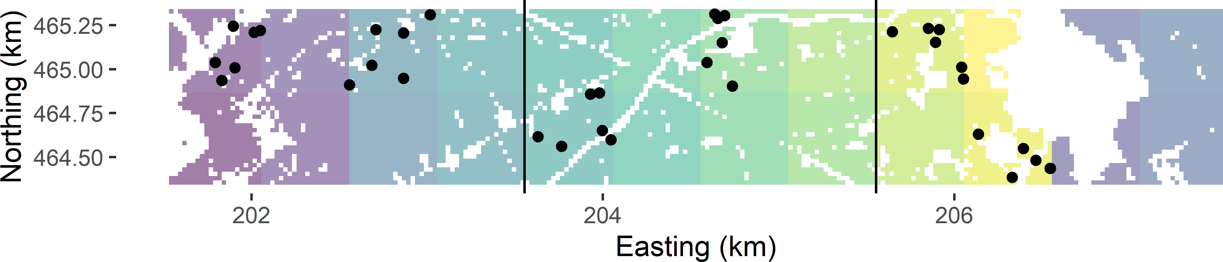
The basic sampling designs stratified random sampling (Chapter 4) and two-stage cluster random sampling can be combined into stratified two-stage cluster random sampling. Figure 7.3 shows a stratified two-stage cluster random sample from Voorst. The strata are groups of eight PSUs within 2 km \(\times\) 1 km blocks, as before in stratified cluster random sampling (Figure 6.2). The PSUs are 0.5 km squares (built-up areas, roads, etc. excluded), as before in (unstratified) two-stage cluster random sampling (Figure 7.1). Within each stratum two times a PSU is selected by ppswr, and every time a PSU is selected, six SSUs (points) are selected by simple random sampling. The stratification avoids the clustering of the selected PSUs in one part of the study area. Compared to (unstratified) two-stage cluster random sampling, the geographical spreading of the PSUs is somewhat improved, which may lead to an increase of the precision of the estimated population mean.
n_h <- rep(2, 3)
m <- 6
set.seed(314)
stratumlabels <- unique(grdVoorst$zone_stratum)
mysample <- NULL
for (i in 1:3) {
  grd_h <- grdVoorst[grdVoorst$zone_stratum == stratumlabels[i], ]
  mysample_h <- twostage(sframe = grd_h, psu = "psu", n = n_h[i], m = m)
  mysample <- rbind(mysample, mysample_h)
}
mysample$s1 <- jitter(mysample$s1, amount = cell_size / 2)
mysample$s2 <- jitter(mysample$s2, amount = cell_size / 2)
The population mean can be estimated in much the same way as with stratified cluster random sampling. With function svymean this is an easy task.
N_h <- tapply(grdVoorst$psu, INDEX = grdVoorst$zone_stratum,
  FUN = function(x) {
    length(unique(x))
    })
M_h <- tapply(grdVoorst$z, INDEX = grdVoorst$zone_stratum, FUN = length)
mysample$w1 <- N_h[mysample$zone_stratum]
mysample$w2 <- M_h[mysample$zone_stratum]
design_str2stage <- svydesign(id = ~ psudraw, strata = ~ zone_stratum,
  weights = ~ w1 + w2, data = mysample, nest = TRUE)
svymean(~ z, design_str2stage)
    mean     SE
z 66.411 4.1335