Chapter 12 Computing the required sample size
An important decision in designing sampling schemes is the number of units to select. In other words, what should the sample size be? If a certain budget is available for sampling, we can determine the affordable sample size from this budget. A costs model is then needed.
The alternative to deriving the affordable sample size from the budget is to start from a requirement on the quality of the survey result obtained by statistical inference. Two types of inference are distinguished, estimation and testing. The required sample size depends on the type of sampling design. With stratified random sampling, we expect that we need fewer sampling units compared to simple random sampling to estimate the population mean with the same precision, whereas with cluster random sampling and two-stage cluster random sampling in general we need more sampling units. To compute the sample size given some quality requirement, we may start with computing the required sample size for simple random sampling and then correct this sample size to account for the design effect. Therefore, I start with presenting formulas for computing the required sample size for simple random sampling. Section 12.4 describes how the required sample sizes for other types of sampling design can be derived.
Hereafter, formulas for computing the required sample size are presented for simple random sampling with replacement of finite populations and simple random sampling of infinite populations. For simple random sampling without replacement (SI) of finite populations, these sample sizes can be corrected by (Lohr 1999)
\[\begin{equation} n_{\mathrm{SI}} = \frac{n_{\mathrm{SIR}}}{1+\frac{n_{\mathrm{SIR}}}{N}} \;, \tag{12.1} \end{equation}\]
with \(n_{\mathrm{SIR}}\) the required sample size for simple random sampling with replacement.
12.1 Standard error
A first option is to set a limit on the variance of the \(\pi\) estimator of the population mean, see Equation (3.7), or on the square root of this variance, the standard error of the estimator. Given a chosen limit for the standard error \(se_{\mathrm{max}}\), the required sample size for simple random sampling with replacement can be computed by
\[\begin{equation} n = \left(\frac{S^*(z)}{se_{\mathrm{max}}}\right)^2 \;, \tag{12.2} \end{equation}\]
with \(S^*(z)\) a prior estimate of the population standard deviation. The required sample size \(n\) should be rounded to the nearest integer greater than the right-hand side of Equation (12.2). This also applies to the following equations.
For the population proportion (areal fraction) as the parameter of interest, the required sample size can be computed by (see Equation (3.14))
\[\begin{equation} n = \left(\frac{\sqrt{p^*(1-p^*)}}{se_{\mathrm{max}}}\right)^2+1 \;, \tag{12.3} \end{equation}\]
with \(p^*\) a prior estimate of the population proportion.
Alternatively, we may require that the relative standard error, i.e., the standard error of the estimator divided by the population mean, may not exceed a given limit \(rse_{\mathrm{max}}\). In this case the required sample size can be computed by
\[\begin{equation} n = \left(\frac{cv^*}{rse_{\mathrm{max}}}\right)^2 \;, \tag{12.4} \end{equation}\]
with \(cv^*\) a prior estimate of the population coefficient of variation \(S(z)/\bar{z}\). For a constraint on the relative standard error of the population proportion estimator, we obtain
\[\begin{equation} n = \left(\frac{p^*(1-p^*)}{rse_{\mathrm{max}}\;p^*}\right)^2+1=\left(\frac{1-p^*}{rse_{\mathrm{max}}}\right)^2+1 \;. \tag{12.5} \end{equation}\]
12.2 Length of confidence interval
Another option is to require that the length of the confidence interval of the population mean may not exceed a given limit \(l_{\mathrm{max}}\):
\[\begin{equation} 2 \; t_{\alpha/2,n-1}\frac{S(z)}{\sqrt{n}} \leq l_{\mathrm{max}} \;, \tag{12.6} \end{equation}\]
with \(t_{\alpha/2,n-1}\) the \((1-\alpha/2)\) quantile of the t distribution with \(n-1\) degrees of freedom, \(S(z)\) the population standard deviation of the study variable, and \(n\) the sample size. The problem is that we do not know the degrees of freedom (we want to determine the sample size \(n\)). Therefore, \(t_{\alpha/2,n-1}\) is replaced by \(u_{\alpha/2}\), the \((1-\alpha/2)\) quantile of the standard normal distribution. Rearranging yields
\[\begin{equation} n = \left(u_{\alpha/2}\frac{S^*(z)}{l_{\mathrm{max}}/2}\right)^2 \;. \tag{12.7} \end{equation}\]
The requirement can also be formulated as
\[\begin{equation} P(|\hat{\bar{z}}-\bar{z}| \leq d_{\mathrm{max}}) \leq 1-\alpha \;, \tag{12.8} \end{equation}\]
with \(d_{\mathrm{max}}\) the margin of error: \(d_{\mathrm{max}}=l_{\mathrm{max}}/2\).
An alternative is to require that with a large probability \(1-\alpha\) the absolute value of the relative error of the estimated mean may not exceed a given limit \(r_{\mathrm{max}}\). In formula:
\[\begin{equation} P\left(\frac{\lvert\hat{\bar{z}}-\bar{z}\rvert}{\bar{z}} \leq r_{\mathrm{max}}\right) \leq 1-\alpha \;. \tag{12.9} \end{equation}\]
Noting that the absolute error equals \(r_{\mathrm{max}} \bar{z}\) and inserting this in Equation (12.7) gives
\[\begin{equation} n = \left(u_{\alpha/2}\frac{cv^*}{r_{\mathrm{max}}}\right)^2 \;. \tag{12.10} \end{equation}\]
As an example, the required sample size is computed for estimating the population mean of the soil organic matter concentration in Voorst. The requirement is that with a probability of 95% the absolute value of the relative error does not exceed 10%. A prior estimate of 0.5 for the population coefficient of variation is used.
cv <- 0.5
rmax <- 0.1
u <- qnorm(p = 1 - 0.05 / 2, mean = 0, sd = 1)
n <- ceiling((u * cv / rmax)^2)
The required sample size is 97. The same result is obtained with function nContMoe of package PracTools (Valliant, Dever, and Kreuter (2021), Valliant, Dever, and Kreuter (2018)).
[1] 9712.2.1 Length of confidence interval for a proportion
Each of the methods for computing a confidence interval of a proportion described in Subsection 3.3.1 can be used to compute the required sample size given a limit for the length of the confidence interval of a proportion. The most simple option is to base the required sample size on the Wald interval (Equation (3.17)), so that the required sample size can be computed by
\[\begin{equation} n = \left(u_{\alpha/2}\frac{\sqrt{p^*(1-p^*)}}{l_{\mathrm{max}}/2}\right)^2 +1\;. \tag{12.11} \end{equation}\]
The Wald interval approximates the discrete binomial distribution by a normal distribution. See the rule of thumb in Subsection 3.3.1 for when this approximation is reasonable.
Package binomSamSize (Höhle 2017) has quite a few functions for computing the required sample size. Function ciss.wald uses the normal approximation. In the next code chunk, the required sample sizes are computed for a prior estimate of the population proportion \(p^*\) of 0.2.
d in the functions below is half the length of the confidence interval.
library(binomSamSize)
p_prior <- 0.2
n_prop_wald <- ciss.wald(p0 = p_prior, d = 0.1, alpha = 0.05)
n_prop_agrcll <- ciss.agresticoull(p0 = p_prior, d = 0.1, alpha = 0.05)
n_prop_wilson <- ciss.wilson(p0 = p_prior, d = 0.1, alpha = 0.05)
The required sample sizes are 62, 58, and 60, for the Wald, Agresti-Coull, and Wilson approximation of the binomial proportion confidence interval, respectively. The required sample size with function ciss.wald is one unit smaller than as computed with Equation (12.11), as shown in the code chunk below.
[1] 6312.3 Statistical testing of hypothesis
The required sample size for testing a population mean with a two-sided alternative hypothesis can be computed by (Ott and Longnecker 2015)
\[\begin{equation} n = \frac{S^2(z)}{\Delta^2}\;(u_{\alpha/2}+u_{\beta})^2 \;, \tag{12.12} \end{equation}\]
with \(\Delta\) the smallest relevant difference of the population mean from the test value, \(\alpha\) the tolerable probability of a type I error, i.e., the probability of rejecting the null hypothesis when the population mean is equal to the test value, \(\beta\) the tolerable probability of a type II error, i.e., the probability of not rejecting the null hypothesis when the population mean is not equal to the test value, \(u_{\alpha/2}\) as before, and \(u_{\beta}\) the \((1-\beta)\) quantile of the standard normal distribution. The quantity \(1-\beta\) is the power of a test: the probability of correctly rejecting the null hypothesis. For a one-sided test, \(u_{\alpha/2}\) must be replaced by \(u_{\alpha}\).
In the next code chunk, the sample size required for a given target power is computed with the standard normal distribution (Equation (12.12)), as well as with the t distribution using function pwr.t.test of package pwr (Champely 2020)6. This requires some iterative algorithm, as the degrees of freedom of the t distribution are a function of the sample size. The required sample size is computed for a one-sample test and a one-sided alternative hypothesis.
library(pwr)
sd <- 4; delta <- 1; alpha <- 0.05; beta <- 0.2
n_norm <- (sd / delta)^2 * (qnorm(1 - alpha) + qnorm(1 - beta))^2
n_t <- pwr.t.test(
  d = delta / sd, sig.level = alpha, power = (1 - beta),
  type = "one.sample", alternative = "greater")
In this example, the required sample size computed with the t distribution is two units larger than that obtained with the standard normal distribution: 101 vs. 99. Package pwr has various functions for computing the power of a test given the sample size, or reversely, the sample size for a given power, such as for the two independent samples t test, binomial test (for one proportion), test for two proportions, etc.
12.3.1 Sample size for testing a proportion
For testing a proportion, a graph is computed with the power of a binomial test against the sample size. This is illustrated with a one-sided alternative \(H_a: p > 0.20\) and a smallest relevant difference of 0.10.
p_test <- 0.20; alpha <- 0.10; delta <- 0.10
n <- 1:150
power <- k_min <- numeric(length = length(n))
for (i in seq_len(length(n))) {
  k_min[i] <- qbinom(p = 1 - alpha, size = n[i], prob = p_test)
  power[i] <- pbinom(
    q = k_min[i], size = n[i], prob = p_test + delta, lower.tail = FALSE)
}
As can be seen in the R code, as a first step for each total sample size the smallest number of successes \(k_{\mathrm{min}}\) is computed at which the null hypothesis is rejected. Then the binomial probability is computed of \(k_{\mathrm{min}}+1\) or more successes for a probability of success equal to \(p_{\mathrm{test}}+\Delta\). Note that there is no need to add 1 to k_min as with argument lower.tail = FALSE the value specified by argument q is not included.
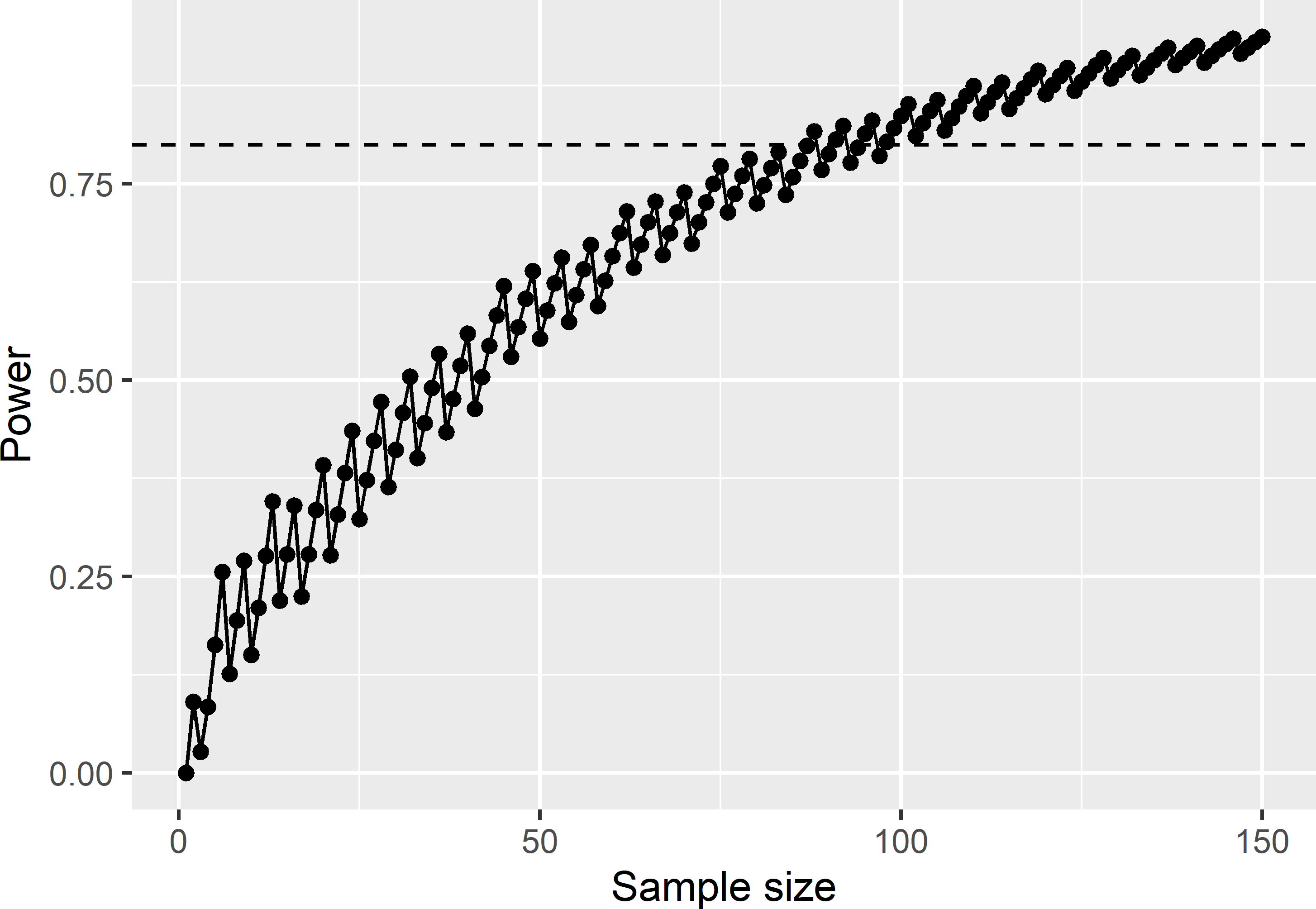
Figure 12.1: Power of right-tail binomial test (test proportion: 0.2; significance level: 0.10).
Figure 12.1 shows that the power does not increase monotonically with the sample size. The graph shows a saw-toothed behaviour. This is caused by the stepwise increase of the critical number of successes (k_min) with the total sample size.
The required sample size can be computed in two ways. The first option is to compute the smallest sample size for which the power is larger than or equal to the required power \(1-\beta\). The alternative is to compute the smallest sample size for which the power is larger than or equal to \(1-\beta\) for all sample sizes larger than this.
n1 <- min(n[which(power > 1 - beta)])
ind <- (power > 1 - beta)
for (i in seq_len(length(n))) {
  if (ind[length(n) - i] == FALSE)
    break
}
n2 <- n[length(n) - i + 1]
The smallest sample size at which the desired level of 0.8 is reached is 88. However, as can be seen in Figure 12.1, for sample sizes 89, 90, 93, 94, and 97, the power drops below the desired level of 0.80. The smallest sample size at which the power stays above the level of 0.8 is 98.
Alternatively, we may use function pwr.p.test of package pwr. This is an approximation, using an arcsine transformation of proportions. The first step is to compute Cohen’s \(h\), which is a measure of the distance between two proportions: \(h = 2\;arcsin(\sqrt{p_1})-2\;arcsin(\sqrt{p_2})\). This can be done with function ES.h. The value of \(h\) must be positive, which is achieved when the proportion specified by argument p1 is larger than the proportion specified by argument p2.
h <- ES.h(p1 = 0.30, p2 = 0.20)
n_approx <- pwr.p.test(
  h, power = (1 - beta), sig.level = alpha, alternative = "greater")
The approximated sample size equals 84, which is somewhat smaller than the required sample sizes computed above.
Exercises
- Write an R script to compute the required sample size, given a requirement in terms of the half-length of the confidence interval of a population proportion. Use a normal approximation for computing the confidence interval. Use a range of values for half the length of the interval: \(d = (0.01, 0.02, \dots , 0.49)\). Use a prior (anticipated) proportion of 0.1 and a significance level of 0.95. Plot the required sample size against \(d\). Explain what you see. Why is it needed to provide a prior proportion?
- Do the same for a single value for the half-length of the confidence interval of 0.2 and a range of values for the prior proportion \(p^* = (0.01,0.02, \dots ,0.49)\). Explain what you see. Why is it not needed to compute the required sample size for prior proportions \(>0.5\)?
12.4 Accounting for design effect
The required sample sizes computed in the previous sections are all for simple random sampling in combination with the \(\pi\) estimator of the population mean. But what is the required sample size for other types of sampling design, such as stratified (simple) random sampling, systematic random sampling, two-stage cluster random sampling, and cluster random sampling? Broadly speaking, we expect that with stratified random sampling and systematic random sampling the sampling variance of the estimator of the mean will be smaller than with simple random sampling of the same number of units, whereas with two-stage cluster random sampling and cluster random sampling we expect larger sampling variances. Therefore, reversely, for the first two types of sampling design, we expect that the sample size required to achieve the same level of accuracy or confidence will be smaller than with simple random sampling, and for the latter two design types this sample size will be larger. The design effect is commonly quantified by the ratio of two sampling variances of the population mean estimator (Lohr 1999):
\[\begin{equation} de(p,\hat{\bar{z}}) = \frac{V_p(\hat{\bar{z}})}{V_{\mathrm{SI}}(\hat{\bar{z}}_{\pi})}= \frac{V_p(\hat{\bar{z}})}{S^2(z)/n}\;, \tag{12.13} \end{equation}\]
with \(V_p(\hat{\bar{z}})\) the sampling variance of an estimator (\(\pi\) estimator, regression estimator) of the population mean with sampling design \(p\) and \(V_{\mathrm{SI}}(\hat{\bar{z}}_{\pi})\) the sampling variance of the \(\pi\) estimator of the population mean with simple random sampling. Given an estimate of this design effect, the required sample size for a more complex sampling strategy (combination of sampling design and estimator), given a constraint on the standard error or the half-length of a confidence interval, can be computed by
\[\begin{equation} n(p,\hat{\bar{z}}) = \sqrt{de(p,\hat{\bar{z}})} \; n(\mathrm{SI},\pi) \;. \tag{12.14} \end{equation}\]
12.5 Bayesian sample size determination
A serious drawback of the classical frequentist approach of computing the required sample size explained in the previous sections is that the required sample sizes are sensitive to the design parameters \(S^*\), \(p^*\), and \(cv^*\). We are rather uncertain about these parameters, and therefore it is attractive to replace a single value for these parameters by a probability distribution. This leads to a different statistical approach of computing the required sample size, the Bayesian approach. This Bayesian approach also offers the possibility of accommodating existing information about the population mean or proportion. In this section I show how this approach can be used to compute the required sample size for estimating a population mean or proportion.
But before going into details, let me explain the basics of the Bayesian approach of statistical inference. In the previous sections, the statistical inference was from the frequentist perspective. How does the frequency distribution of the estimator of the population mean look like if we repeat the selection of a sample with a given sampling design? Is the mean of this frequency distribution, referred to as the sampling distribution, equal to the population mean, and what is the variance of this sampling distribution?
The Bayesian approach is fundamentally different. The frequency distribution of the frequentist approach is replaced by a probability distribution of the population mean reflecting our belief about the population mean. Note that expressing our belief in terms of a probability distribution implies that in the Bayesian approach, contrary to the frequentist approach, the population mean is a random variable. Where in the frequentist approach, it is incorrect to say that the probability that the population mean is inside the 95% confidence interval equals 95% (see Section 3.3), this is perfectly fine in the Bayesian approach. The term confidence interval is replaced by the term credible interval to underline the fundamental different meaning of the interval.
The first step in the Bayesian approach of statistical inference is to postulate a prior distribution for the population parameter of interest. This prior distribution expresses our belief and uncertainty about the parameter before the sample data are taken into account.
The next step is to formalise a theory about the data. This boils down to making an assumption about the type of distribution function of the data. Can we safely assume that the data follow a normal or a binomial distribution? Once the type of distribution has been specified, we can write an equation for the probability of the data as a function of the parameter. This function is referred to as the likelihood function.
The final step is to revise our prior belief about the population parameter of interest, using the data and our theory about the data as expressed in the likelihood function. This results in the posterior distribution of the parameter. Our revised or updated belief is computed with Bayes’ rule:
\[\begin{equation} f(\theta|\mathbf{z}) = \frac{f(\theta) f(\mathbf{z}|\theta)} {f(\mathbf{z})}\;, \tag{12.15} \end{equation}\]
with \(f(\theta|\mathbf{z})\) the posterior distribution, i.e., the probability density7 of the parameter given the sample data, \(f(\theta)\) our prior belief in the parameters specified by a probability distribution (prior distribution), \(f(\mathbf{z}|\theta)\) the likelihood of the data, and \(f(\mathbf{z})\) the probability distribution of the data.
12.5.1 Bayesian criteria for sample size computation
Equation (12.15) shows that the posterior distribution of the population parameter of interest depends on the probability distribution of the new data \(f(\mathbf{z})\). The problem is that these new data are not yet known. We are designing a sample, and the data yet are to be collected, so at first glance this might seem an unsolvable problem. However, what we could do is to simulate with the prior probability density function a large number of values of the population parameter(s), and with each parameter a large number of possible vectors with \(n\) data. Each data vector is then used to update the prior to the posterior, using Bayes’ rule (Equation (12.15)). For each posterior either the length of the highest posterior density (HPD) interval with a coverage probability of \(1-\alpha\) is computed, or reversely, the coverage probability of the HPD interval of length \(l_{\mathrm{max}}\). Finally, the average of the lengths of the HPD intervals or the average of the coverage probabilities is computed, and these averages are compared with our precision requirement. If the average length is larger than \(l_{\mathrm{max}}\), or the coverage probability of intervals of length \(l_{\mathrm{max}}\) is smaller than \(1-\alpha\), then we must increase \(n\); if the average length is smaller than \(l_{\mathrm{max}}\), or the coverage probability of intervals of length \(l_{\mathrm{max}}\) is larger than \(1-\alpha\), then we must decrease \(n\). This whole procedure is repeated until our precision requirement is met. Simulation is one option to compute the sample size, (partly) analytical approaches are also available.
More formally, the procedure is as follows. The prior probability density function on the population parameter(s) \(\theta\) is used to compute for a given sample size \(n\) the predictive distribution of the data:
\[\begin{equation} f(\mathbf{z}|n) = \int_{\Theta} f(\mathbf{z}|\theta,n)f(\theta)\mathrm{d}\theta\;, \tag{12.16} \end{equation}\]
with \(\Theta\) the parameter space for \(\theta\) containing all possible values of \(\theta\). This predictive distribution is also named the preposterior distribution, stressing that the data are not yet accounted for in the distribution.
Even if \(\theta\) would be fixed, we do not have only one vector \(\mathbf{z}\) with \(n\) data values but a probability distribution, from which we can simulate possible data vectors, referred to as the data space \(\mathcal{Z}\). In case of a binomial probability and sample size \(n\), the data space \(\mathcal{Z}\) (in the form of the number of observed successes given sample size \(n\)) can be written as the set \(\{0,1,\dots,n\}\), i.e., one vector of length \(n\) with all “failures”, \(n\) vectors of length \(n\) with one success, \({n \choose 2}\) vectors with two successes, etc. Each data vector is associated with a probability density (for continuous data) or probability mass (for discrete data). As a consequence, we do not have only one posterior distribution function \(f(\theta|\mathbf{z})\), but as many as we have data vectors in the data space. For each posterior distribution function the coverage of the HPD interval of a given length can be computed, or reversely, the length of the HPD interval for a given coverage. This leads to various criteria for computing the required sample size, among which are the average length criterion (ALC), the average coverage criterion (ACC), and the worst outcome criterion (WOC) (L. Joseph, Wolfson, and du Berger (1995), L. Joseph and Bélisle (1997)).
12.5.1.1 Average length criterion
For a fixed posterior HPD interval coverage of \(100(1-\alpha)\)%, the smallest sample size \(n\) is determined such that
\[\begin{equation} \int_{\mathcal{Z}} l(\mathbf{z},n) f(\mathbf{z}|n)\mathrm{d}\mathbf{z} \leq l_{\mathrm{max}}\;, \tag{12.17} \end{equation}\]
where \(f(\mathbf{z}|n)\) is the predictive distribution of the data (Equation (12.16)) and \(l(\mathbf{z},n)\) is the length of the \(100(1-\alpha)\)% HPD interval for data \(\mathbf{z}\) and sample size \(n\), obtained by solving
\[\begin{equation} \int_v^{v+l(\mathbf{z},n)}f(\theta|\mathbf{z},n)\mathrm{d}\theta= 1-\alpha\;, \tag{12.18} \end{equation}\]
for \(l(\mathbf{z},n)\), for each possible data set \(\mathbf{z} \in \mathcal{Z}\). \(f(\theta|\mathbf{z},n)\) is the posterior density of the population parameter of interest given the data \(\mathbf{z}\) and sample size \(n\). ALC ensures that the average length of \(100(1-\alpha)\)% posterior HPD intervals, weighted by \(f(\mathbf{z}|n)\), is at most \(l_{\mathrm{max}}\).
12.5.1.2 Average coverage criterion
For a fixed posterior HPD interval of length \(l_\mathrm{max}\), the smallest sample size \(n\) is determined such that
\[\begin{equation} \int_{\mathcal{Z}} \left\{ \int_v^{v+l_\mathrm{max}}f(\theta|\mathbf{z},n)\mathrm{d}\theta \right\} f(\mathbf{z}|n)\mathrm{d}\mathbf{z} \geq 1-\alpha \;. \tag{12.19} \end{equation}\]
ACC ensures that the average coverage of HPD intervals of length \(l_\mathrm{max}\) is at least \(1-\alpha\). The integral inside the curly brackets is the integral of the posterior density of the population parameter of interest over the HPD interval \((v,v+l_\mathrm{max})\), given a data vector \(\mathbf{z}\) of size \(n\). The mean of this integrated posterior density of the parameter of interest \(\theta\) is obtained by multiplying the integrated density with the predictive probability of the data and integrating over all possible data sets in \(\mathcal{Z}\).
12.5.1.3 Worst outcome criterion
Neither ALC nor ACC guarantee that for a particular data set \(\mathbf{z}\) the criterion is met, as both are defined as averages over all possible data sets in \(\mathcal{Z}\). A more conservative sample size can be computed by requiring that for all data sets \(\mathcal{Z}\) both criteria are met. L. Joseph and Bélisle (1997) modified this criterion by restricting the data sets to a subset \(\mathcal{W}\) of most likely data sets. The criterion thus obtained is referred to as the modified worst outcome criterion, or for short, the worst outcome criterion (WOC). So, the criterion is
\[\begin{equation} \mathrm{inf}_{\mathbf{z} \in \mathcal{W}} \left\{\int_v^{v+l(\mathbf{z},n)}f(\theta|\mathbf{z},n)\mathrm{d}\theta\right\} \geq 1- \alpha \;. \tag{12.20} \end{equation}\]
The smallest sample size satisfying this condition is used as the sample size. For instance, if the 95% most likely data sets are chosen as subspace \(\mathcal{W}\), WOC guarantees that there is 95% assurance that the length of the \(100(1-\alpha)\)% posterior HPD intervals will be at most \(l_{\mathrm{max}}\). The fraction of most likely data sets in subspace \(\mathcal{W}\) is referred to as the worst level.
12.5.2 Mixed Bayesian-likelihood approach
Besides the fully Bayesian approach, L. Joseph and Bélisle (1997) describe a mixed Bayesian-likelihood approach for determining the sample size. In the mixed Bayesian-likelihood approach of sample size determination, the prior distribution of the parameter or parameters is only used to derive the predictive distribution of the data (Equation (12.16)), not the posterior distributions of the parameter of interest for each data vector. For analysis of the posterior distribution, an uninformative prior is therefore used. This mixed approach is of interest when, after the data have been collected, we prefer to estimate the population mean from these data only, using the frequentist approach described in previous sections.
An example of a situation where the mixed Bayesian-likelihood approach can be attractive is the following. Suppose some data of the study variable from the population of interest are already available, but we would like to collect more data so that we will be more confident about the (current) population mean once these new data are collected. The legacy data are used to construct a prior distribution. We have doubts about the quality of the legacy data because they were collected a long time ago and the study variable might have changed in the meantime. In that case, the mixed Bayesian-likelihood approach can be a good option – we are willing to use the legacy data to plan the sampling, but not to make statements about the current population.
No closed formula for computing the required sample size exists for this approach because the posterior density function \(f(\theta|z,n)\) is not a well-defined distribution as before. However, the required sample size still can be approximated by simulation.
12.5.3 Estimation of population mean
The three criteria (ALC, ACC, and WOC) described above are now used to compute the required sample size for estimating the population mean, assuming that the data come from a normal distribution. As we are uncertain about the population standard deviation \(\sigma\) (\(S^*(z)\) in Equation (12.7) is only a prior point estimate of \(\sigma\)), a prior distribution is assigned to this parameter. It is convenient to assign a gamma distribution as a prior distribution to the reciprocal of the population variance, referred to as the precision parameter \(\lambda = 1/\sigma^2\). More precisely, a prior bivariate normal-gamma distribution is assigned to the population mean and the precision parameter8. With this prior distribution, the posterior distribution of the population mean is fully defined, i.e., both the type of distribution and its parameters are known. The prior distribution is so-called conjugate with the normal distribution.
The gamma distribution has two parameters: \(a\) and \(b\). Figure 12.2 shows the gamma distribution for \(a=5\) and \(b=100\).
a <- 5; b <- 100
x <- seq(from = 0, to = 0.2, length = 1000)
dg <- dgamma(x = x, shape = a, scale = 1 / b)
plot(x = x, y = dg, type = "l", ylab = "Density", xlab = "Precision")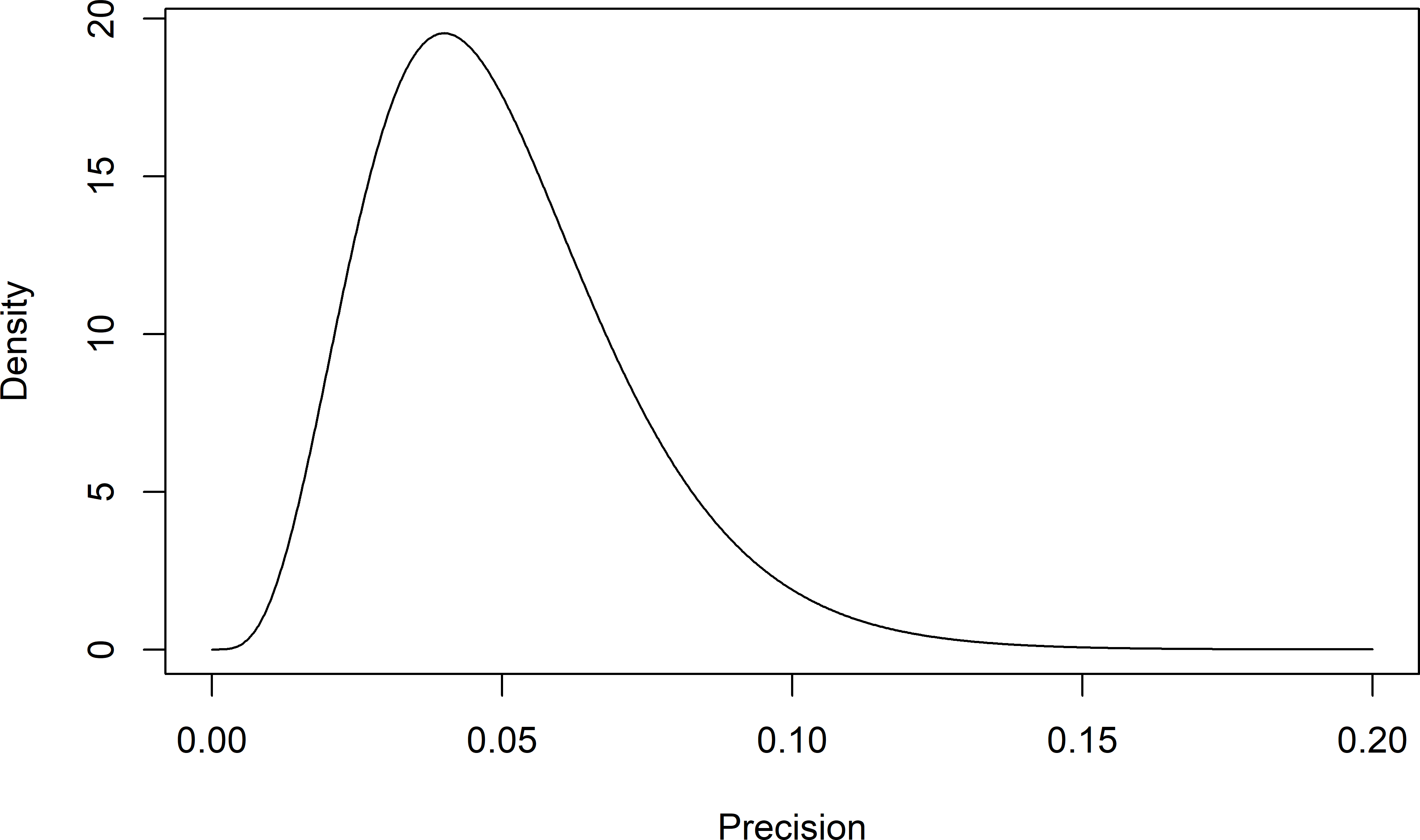
Figure 12.2: Prior gamma distribution for the precision parameter for a shape parameter \(a=5\) and a scale parameter \(1/b=1/100\).
The mean of the precision parameter \(\lambda\) is given by \(a/b\) and its standard deviation by \(\sqrt{a/b^2}\).
The normal-gamma prior is used to compute the predictive distribution for the data. For ACC the required sample size can then be computed with (Adcock 1988)
\[\begin{equation} n = \frac{4b}{a\; l_{\mathrm{max}}^2}t^2_{2a;\alpha/2} - n_0 \;, \tag{12.21} \end{equation}\]
with \(t^2_{2a;\alpha/2}\) the squared \((1-\alpha/2)\) quantile of the (usual, i.e., neither shifted nor scaled) t distribution with \(2a\) degrees of freedom and \(n_0\) the number of prior points. The prior sample size \(n_0\) is only relevant if we have prior information about the population mean and an informative prior is used for this population mean. If we have no information about the population mean, a non-informative prior is used and \(n_0\) equals 0. Note that as \(a/b\) is the prior mean of the inverse of the population variance, Equation (12.21) is similar to Equation (12.7). The only difference is that a quantile from the standard normal distribution is replaced by a quantile from a t distribution with \(2a\) degrees of freedom.
No closed-form formula exists for computing the smallest \(n\) satisfying ALC, but the solution can be found by a bisectional search algorithm (L. Joseph and Bélisle 1997).
Package SampleSizeMeans (L. Joseph and Bélisle 2012) is used to compute Bayesian required sample sizes, using both criteria, ACC and ALC, for the fully Bayesian and the mixed Bayesian-likelihood approach. The gamma distribution plotted in Figure 12.2 is used as a prior distribution for the precision parameter \(\lambda\). As a reference, also the frequentist required sample size is computed.
library(SampleSizeMeans)
lmax <- 2
n_freq <- mu.freq(len = lmax, lambda = a / b, level = 0.95)
n_alc <- mu.alc(len = lmax, alpha = a, beta = b, n0 = 0, level = 0.95)
n_alcmbl <- mu.mblalc(len = lmax, alpha = a, beta = b, level = 0.95)
n_acc <- mu.acc(len = lmax, alpha = a, beta = b, n0 = 0, level = 0.95)
n_accmbl <- mu.mblacc(len = lmax, alpha = a, beta = b, level = 0.95)
n_woc <- mu.modwoc(
  len = lmax, alpha = a, beta = b, n0 = 0, level = 0.95, worst.level = 0.95)
n_wocmbl <- mu.mblmodwoc(
len = lmax, alpha = a, beta = b, level = 0.95, worst.level = 0.95)| Freq | ALC | ALC-MBL | ACC | ACC-MBL | WOC | WOC-MBL |
|---|---|---|---|---|---|---|
| 77 | 92 | 93 | 100 | 102 | 194 | 201 |
| Freq: required sample size computed with the frequentist approach; ALC: average length criterion; ACC: average coverage criterion; WOC: worst outcome criterion. |
Table 12.1 shows that all six required sample sizes are larger than the frequentist required sample size. This makes sense, as the frequentist approach does not account for uncertainty in the population variance parameter. The mixed approach leads to slightly larger required sample sizes than the fully Bayesian approach. This is because in the mixed approach the prior distribution of the precision parameter is not used. Apparently, we do not lose much information by ignoring this prior. With WOC the required sample sizes are about twice the sample sizes obtained with the other two criteria, but this depends of course on the size of the subspace \(\mathcal{W}\). If, for instance the 80% most likely data sets are chosen as subspace \(\mathcal{W}\), the required sample sizes are much smaller.
n_woc80 <- mu.modwoc(
  len = lmax, alpha = a, beta = b, n0 = 0, level = 0.95, worst.level = 0.80)
n_wocmbl80 <- mu.mblmodwoc(
  len = lmax, alpha = a, beta = b, level = 0.95, worst.level = 0.80)
The required sample sizes with this criterion are 124 and 128 using the fully Bayesian and the mixed Bayesian-likelihood approach, respectively.
12.5.4 Estimation of a population proportion
The same criteria can be used to estimate the proportion of a population or, in case of an infinite population, the areal fraction, satisfying some condition (L. Joseph, Wolfson, and du Berger 1995). With simple random sampling, this boils down to estimating the probability-of-success parameter \(p\) of a binomial distribution. In this case the space of possible outcomes \(\mathcal{Z}\) is the number of successes, which is discrete: \(\mathcal{Z} = \{0,1,\dots ,n\}\) with \(n\) the sample size.
The conjugate prior for the binomial likelihood is the beta distribution:
\[\begin{equation} p \sim \frac{1}{B(c,d)} \pi^{c-1} (1-\pi)^{d-1} \;, \tag{12.22} \end{equation}\]
where \(B(c,d)\) is the beta function. The two parameters \(c\) and \(d\) correspond to the number of ‘successes’ and ‘failures’ in the problem context. The larger these numbers, the more the prior information, and the more sharply defined the probability distribution. The plot below shows this distribution for \(c=0.6\) and \(d=2.4\).
c <- 0.6; d <- 2.4
x <- seq(from = 0, to = 1, length = 1000)
dbt <- dbeta(x = x, shape1 = c, shape2 = d)
plot(x = x, y = dbt, type = "l", ylab = "Density", xlab = "Proportion")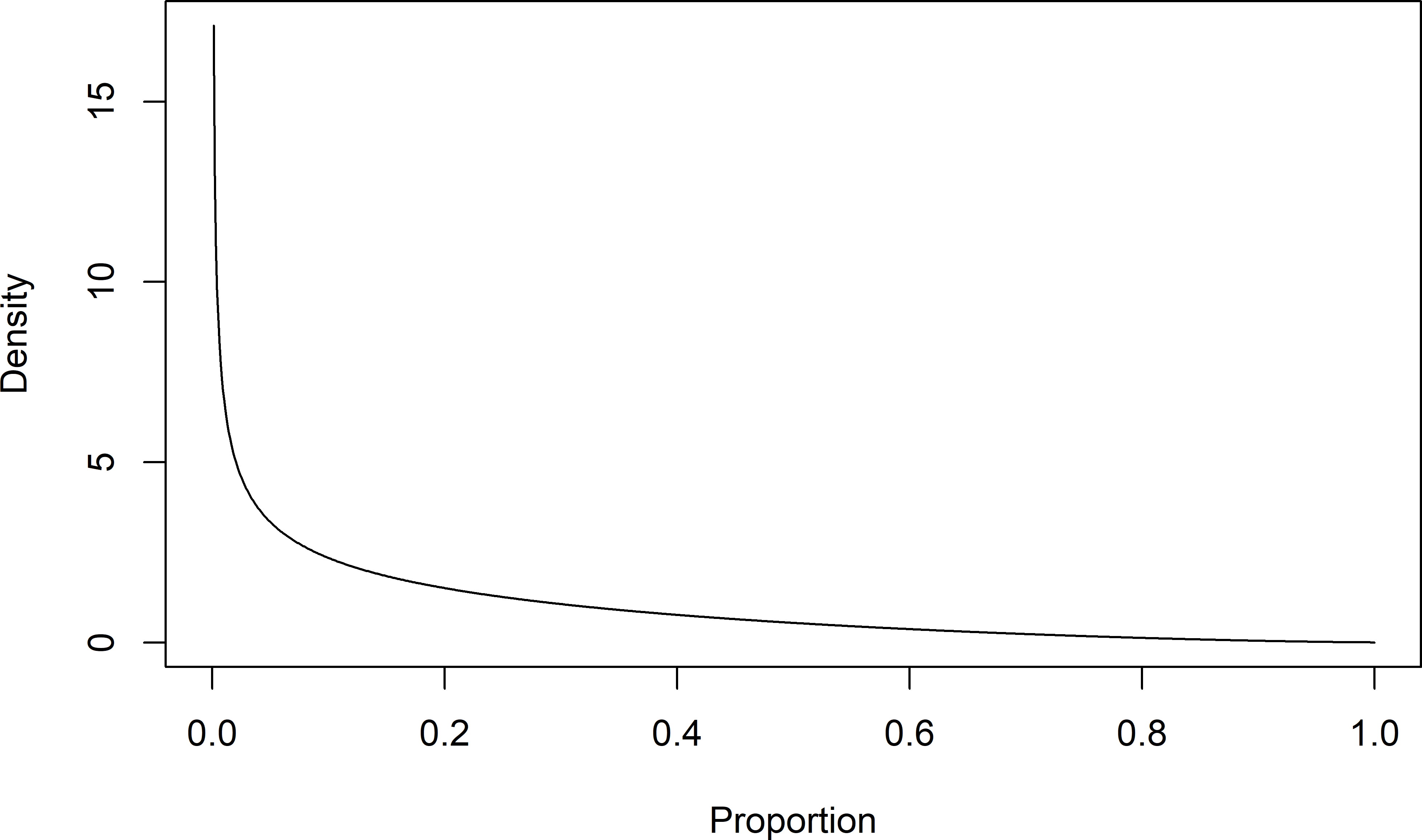
Figure 12.3: Prior beta distribution for the binomial proportion for a beta function \(B(0.6,2.4)\).
The mean of the binomial proportion equals \(c/(c+d)\) and its standard deviation \(\sqrt{cd/\{(c+d+1)(c+d)^2\}}\).
The preposterior marginal distribution of the data is the beta-binomial distribution:
\[\begin{equation} f(z|n) = \binom{n}{z}\frac{B(z+c,n-z+d)}{B(c,d)}\;, \tag{12.23} \end{equation}\]
and for a given number of successes \(z\) out of \(n\) trials the posterior distribution of \(p\) equals
\[\begin{equation} f(p|z,n,c,d)=\frac{1}{B(z+c,n-z+d)} p^{z+c-1} (1-p)^{n-z+d-1} \;. \tag{12.24} \end{equation}\]
For the binomial parameter, criterion ALC (Equation (12.17)) can be written as \[\begin{equation} \sum_{z=0}^n l(z,n)f(z,n) \leq l_{\mathrm{max}} \;. \tag{12.25} \end{equation}\]
To compute the smallest \(n\) satisfying this condition, for each value of \(z\) and each \(n\), \(l(z,n)\) must be computed so that
\[\begin{equation} \int_v^{v+l(z,n)}f(p|z,n,c,d) \mathrm{d}p = 1-\alpha \;, \tag{12.26} \end{equation}\]
with \(v\) the lower bound of the HPD credible set given the sample size and the observed number of successes \(z\).
For the binomial parameter, criterion ACC (Equation (12.19)) can be written as
\[\begin{equation} \sum_{z=0}^n \mathrm{Pr}\{p \in (v,v+l_{\mathrm{max}})\} f(z,n) \geq 1-\alpha \;, \tag{12.27} \end{equation}\]
with
\[\begin{equation} \mathrm{Pr}\{p \in (v,v+l_{\mathrm{max}})\} \propto \int_{v}^{v+l_{\mathrm{max}}}p^z(1-p)^{n-z} f(p) \mathrm{d}p\;, \tag{12.28} \end{equation}\]
with \(f(p)\) the prior density of the binomial parameter.
For more details about ACC and ALC, and about how the required sample size can be computed with WOC in case of the binomial parameter \(p\), refer to L. Joseph, Wolfson, and du Berger (1995).
The required sample sizes for ALC, ACC, and WOC described in the previous subsection, using the fully Bayesian approach or the mixed Bayesian-likelihood approach, can be computed with package SampleSizeBinomial(Lawrence Joseph et al. 2018). This package is used to compute the required sample sizes using the beta distribution shown in Figure 12.3 as a prior for the population proportion. Note that argument len of the various functions of package SampleSizeBinomial specifies the total length of the confidence interval, not half the length as passed to function ciss.wald using argument d.
library(SampleSizeBinomial)
n_alc <- prop.alc(
  len = 0.2, alpha = c, beta = d, level = 0.95, exact = TRUE)$n
n_alcmbl <- prop.mblalc(
  len = 0.2, alpha = c, beta = d, level = 0.95, exact = TRUE)$n
n_acc <- prop.acc(
  len = 0.2, alpha = c, beta = d, level = 0.95, exact = TRUE)$n
n_accmbl <- prop.mblacc(
  len = 0.2, alpha = c, beta = d, level = 0.95, exact = TRUE)$n
n_woc <- prop.modwoc(
  len = 0.2, alpha = c, beta = d, level = 0.95, exact = TRUE,
  worst.level = 0.80)$n
n_wocmbl <- prop.mblmodwoc(
  len = 0.2, alpha = c, beta = d, level = 0.95, exact = TRUE,
  worst.level = 0.80)$n
library(binomSamSize)
n_freq <- ciss.wald(p0 = c / (c + d), d = 0.1, alpha = 0.05)
The required sample sizes are shown in Table 12.2.
| Freq | ALC | ALC-MBL | ACC | ACC-MBL | WOC | WOC-MBL |
|---|---|---|---|---|---|---|
| 62 | 33 | 38 | 50 | 53 | 80 | 81 |
| Freq: required sample size computed with the frequentist approach; ALC: average length criterion; ACC: average coverage criterion; WOC: worst outcome criterion. |